Category Archives: Studio One
Set Up the Quantum Interface Preamps with One Track
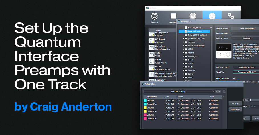
A single Automation track can set up a session’s preamp levels and phantom power in the Quantum interface, as well as the older Studio 192. So, you can stop taking the time to reset preamp levels if you do lots of different sessions—let Studio One set up the preamps whenever you call up a specific song.
For example, I mostly use three vocal mics. However, their optimum gain settings vary for narration, music vocals, or recording my main background vocalist—who needs different gain settings depending on whether she’s doing upfront vocals, or ooohs/ahhhs.
To call up specific preamp levels for different songs, simply create an automation track (or tracks) at the song’s beginning. Then, when you first hit record, the track sets up levels and (with Quantum and Studio 192) phantom power on/off for up to 8 channels. The next time you call up that song, the mics will be at the right levels, with phantom power set as desired. Here’s how to do it.
1. In Universal Control, under MIDI Control, select Internal. Or, choose Enabled if you also want to be able to control Quantum from an external controller.
2. Choose Studio One > Options (Windows) or Preferences (macOS), and select External Devices.
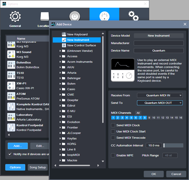
3. Select Add. Choose New Instrument.
4. For Receive From, choose Quantum MIDI In. For Send To, choose Quantum MIDI Out. Also tick MIDI Channels 1 – 8 (fig. 1). Then, click OK.
5. Create an Automation track. To show automation, type keyboard shortcut A.
6. From the track’s automation drop-down menu, click on Add/Remove. In the right pane, unfold the External Devices folder, then unfold the folder for the Channel that corresponds to the preamp you want to control (Channel 1 = Preamp 1, Channel 2 = Preamp 2…Channel 8 = Preamp 8). See fig. 2.
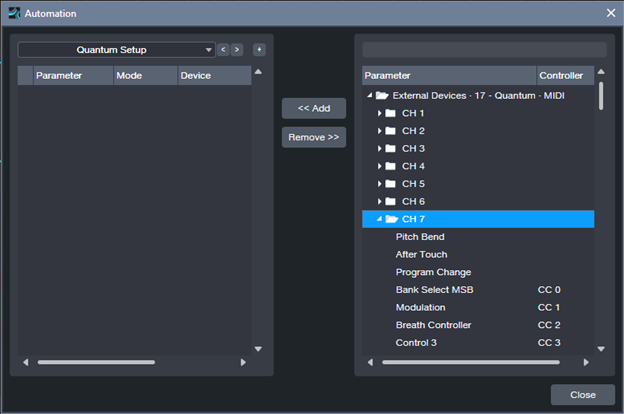
7. For each preamp you want to set up, add CC7 (this controls preamp volume) and CC14 (controls phantom power). For example, I typically set up channels 6, 7, and 8. After adding these continuous controllers, the Automation menu’s right side looks like fig. 3 (except with your specific channel numbers). Click on Close after making your selections.

8. To set up the preamp levels, choose the parameter you want to program in the Automation track’s drop-down menu. Note that in the documentation, the phantom power control settings are reversed. The correct values for CC14 are 0 to 63 = Off, and 64 to 127 = On. To set the preamp level, with Universal Control open, adjust the envelope for the desired preamp gain reading (you can also see the level on the Quantum’s display).
9. Set the initial level and phantom power parameter values for the chosen preamps. Now your automation track will reproduce those settings, exactly as programmed, the next time you open the song. Given that I do voiceover or narration for at least one video a week, I can’t tell you how much time that saves—I load my narration template, and don’t even have to think about adjusting levels before hitting record.
Getting Fancy
A cool trick is to reserve a song’s first measure for doing the setup. Turn on phantom power at the song start, but fade up the volume to the desired level after the phantom power is on. That avoids power-on spikes from the mics. However, when adjusting the level envelope, the preamp knobs change only if you adjust the left-most node. So, set the preamp level you want with this node, then move it to the right on the timeline. Create another node at 0 that fades up to the node you moved, which sets the final volume.
Another trick is to have more than one automation track. For example, on most songs I have a setup track for me, and a setup track for the background singer. When she does overdubs, I turn my automation track to Off, and set her automation track to Read so it sets her levels.
Coda: Windows Meets Thunderbolt
The first time I tried Quantum on a Mac, it worked perfectly. With Windows, well…it’s Windows. My computer is a PC Audio Labs Rok Box (great machine, by the way) with dual Thunderbolt 3 ports. I used Apple’s TB3-to-TB2 adapter—no go. I found a new Thunderbolt driver for the motherboard, and asked PC Audio Labs tech support about whether I should install it. They advised doing so, and said if I had problems, they’d bail me out. But after installation, the Quantum’s power button’s color was still Unhappy Red instead of Happy Blue. I was about to contact support again, but stumbled on a program in the computer called Thunderbolt Control Center. I opened it, which showed Quantum was connected—but I hadn’t given the computer “permission” to connect. So, I gave permission. With its new-found freedom, the Quantum burst into its low-latency glory.
The moral of the story: Thunderbolt has many variables on Windows than macOS. But as with life itself, perseverance furthers.
The “Drenched” Chorus
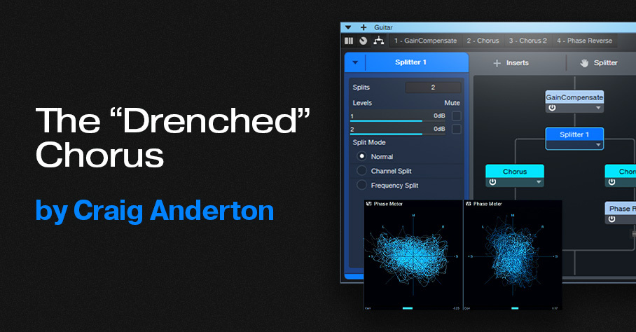
Studio One’s chorus gives the “wet” sound associated with chorus effects. But I wanted a chorus that went beyond wet to drenched—something that could swirl in the background of a thick arrangement, and shower the stereo field like a sprinkler system. Check out the audio example: the first part is the Drenched Chorus, and the second part is the standard Chorus.
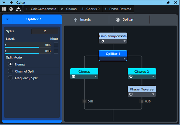
This FX Chain for Studio One Professional (see the download link at the end) supercharges the wet sound by inserting two choruses in parallel, and reversing the phase for one of them (fig. 1). This cancels any dry sound, leaving only the animation from the stereo chorus. A Mixtool provides the phase reversal. Another Mixtool at the input adds gain, to compensate for the level that’s lost through phase cancellation.
The Choruses are essentially set to the default preset, but with Low Freq at minimum and High Freq at maximum for the widest frequency response. Fig. 2 uses a phase meter to compare the Drenched Chorus (left) with the standard Chorus (right), playing the same section of a guitar part. Note how the Drenched Chorus puts a lot of energy into the sides, which accounts for the big stereo image. Meanwhile, the center has less level than the standard chorus, due to any vestiges of dry signal being removed.
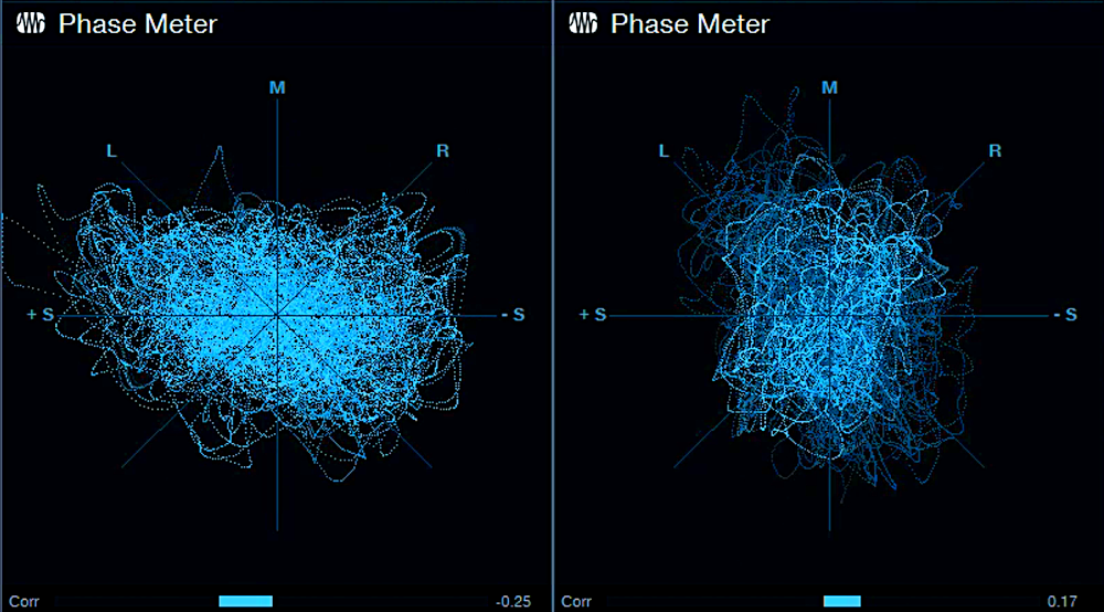
This effect is designed for stereo playback, but note that in fig. 2, the Drenched Chorus’s correlation is negative. Normally you want to avoid this, because audio with negative correlation will cancel when played back in mono. However, the correlation swings wildly between positive and negative, so it’s not much of an issue. With mono playback, all that happens is a slight level loss due to occasional negative correlations. The effect still sounds like a chorus, although of course you lose the cool stereo effects.
How to Use It
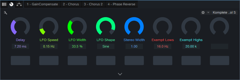
Download the FX Chain, and drag it into a channel’s insert. The Macro Controls (fig. 3) affect only Chorus 2. Here’s what they do:
- Delay: Set this to 9.00 for maximum cancellation. The sound is somewhat like a combination of chorusing and flanging. Offsetting from this time increases the chorus effect. The maximum Drenched Chorus effect occurs between approximately 7 and 11 ms.
- LFO Speed: I prefer settings below 0.30 Hz, but higher settings have a bit of a rotating speaker vibe.
- LFO Width: More Width increases the chorusing effect. If you turn this up, I recommend keeping LFO Speed below 0.30 Hz.
- LFO Shape: Setting this to Triangle uses the same shape as the other Chorus. Sine gives a subtly different sound.
- Stereo Width: Extends the stereo image outward when turned clockwise.
- Exempt Lows: This turns up the Low Freq filter, which reduces cancellation at those frequencies. Use this when you want more of the direct sound instead of maximum drenching.
- Exempt Highs: This turns down the High Freq filter, which reduces cancellation at those frequencies. Personally, I leave both controls all the way down for maximum moisture, but turn them up if you want the track to swim a little less in the background.
Download the FX Chain below!
Solve Vocal Problems with the De-Esser
Studio One offers several ways to “de-ess” excessive sibilants (“s” sounds). De-essing combines compression and EQ. The EQ focuses on the frequency range where sibilants are most prominent. Then, compression reduces this range’s level when sibilants are present. Prior to version 6, using Multiband Dynamics was the best way to do de-essing.
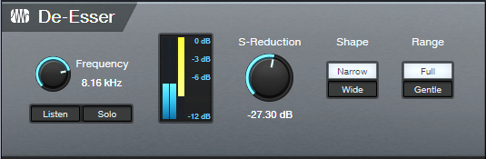
With version 6, the Pro EQ3’s new dynamic EQ functionality is excellent for reducing ess sounds. However, the equally new De-Esser (fig. 1) is designed specifically for the job of fixing excessive sibilance, quickly and effectively.
To get the most out of the De-Esser, note that some of the parameters work together as a team. So, alternating edits between some controls is often the best way to optimize the effect.
Getting Started
Ess sounds tend to be short. By the time you’ve started to tweak a parameter, the ess sound has likely already ended. So, for easy editing, create a short loop on a word with the prominent ess sound.
Frequency and Listen
1. Enable Listen.
2. Vary Frequency until you find the frequency where the ess sound is most prominent.
Solo and S-Reduction
3. After identifying the frequency, enable Solo. You’ll hear only the ess sound whose volume is being reduced.
4. Adjust S-Reduction to get a feel for the optimum ess reduction amount. At 0.00 dB, there’s no reduction. At ‑60.00, sounds in addition to the ess sound will likely be reduced.
5. Next, turn off Solo, and adjust S-Reduction in context with the looped word. Less negative S-Reduction values concentrate on reducing the ess sound’s initial transient. More negative values reduce more of the ess sound past the initial transient.
6. Do a final Frequency parameter check to optimize the high-frequency response with de-essing. For example, you may be able to raise the frequency to retain more highs, yet still have effective ess reduction.
The metering is helpful in optimizing the De-Esser’s settings. The orange meter shows the amount of reduction. The blue meter shows the input level.
How to Use the Shape Parameter
Ess sounds cover a fairly small range of high frequencies. The Narrow Shape is best for this application because it compresses a narrow band. Frequencies above and below that band remain untouched.
In addition to ess sounds, the De-Esser can also reduce “shhh” sounds (e.g., like the shh sound in “action” or “compression”). Shh sounds cover a wider range of frequencies, and often require a lower Frequency setting. For these sounds, the Wide Shape splits the audio into high and low bands, and processes the entire high band.
You may need to do two passes, one with a Wide Shape for shh sounds, and one with a Narrow Shape for ess sounds. Be conservative with the settings for the two passes, because the changes will reinforce each other.
How to Use the Range Parameter
This parameter is the De-Esser’s unsung hero. Setting Range to Full allows the full amount of reduction dialed in by S-Reduction. Gentle Range restricts reduction to ‑6 dB.
The Gentle setting is useful for more than just guaranteeing a subtler effect. With the Gentle Range enabled, you can dial in huge amounts of S-Reduction. This allows processing as much of the ess or shh sound as possible, not just the initial transient. However, limiting the amount of reduction to -6 dB prevents the amount of reduction from being objectionable.
Final Note
The De-Esser is not just for singing, but also podcasts, voiceovers, and narration. It can even reduce harshness with amp sims, as described in De-Esser Meets Amp Sims. And it can probably do other things that are yet to be discovered!
Authentic 60s Flanger for Artist
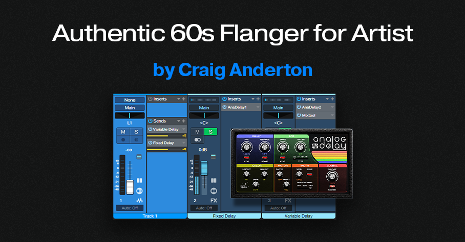
In the 60s, flanging was an electro-mechanical process that involved two turntables or two tape recorders. Since then, flanging has evolved into a digitally driven effect, with a variety of cool bells and whistles. Paradoxically, though, many of today’s digital flangers can’t reproduce the period-correct sound of 60s flanging.
Five years ago, I wrote a blog post about a vintage flanger FX Chain that took advantage of Studio One Pro’s Splitter and Extended FX Chains features. Although this week’s tip takes a little more effort to set up than just loading an FX Chain, and doesn’t have Macro Controls, it gives the same authentic flanging sound for Studio One Artist—check out the audio example.
The 60s flanging sound has three important qualities:
- The flanging effect is controlled manually, not with an LFO. Flanging resulted by manipulating a variable speed option on one of the turntables or tape recorders, or manually pressing on the tape flange or turntable platter to cause a temporary speed change.
- Through-zero flanging. 60s flanging was not a real-time process. One of the turntables or tape recorders could go forward in time, compared to the other one. Typically, one of the audio paths was also switched out of phase. When one path transitioned across the point where it went from being behind the other path to being ahead of it, there was a brief moment when the two signals would cancel. This was called the through-zero point, and contributed to flanging’s dramatic sound.
- Motor inertia. Mechanical motors couldn’t respond instantly to speed changes, so manual flanging was somewhat unpredictable. After changing a tape recorder’s variable speed setting, it would take a while for the motor to catch up. This created a smooth, “liquid” feel as you controlled the flanging effect. The Inertia control in Studio One’s Analog Delay emulates the feel of controlling a mechanical device.
The Setup
Fig. 1 shows the track setup for the flanging effect.
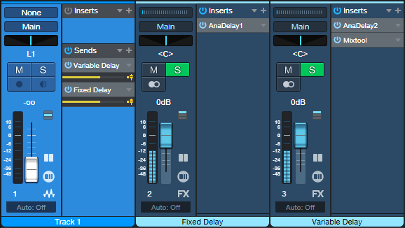
1. The track you want to flange feeds two FX buses via pre-fader Sends. Turn the track’s channel fader down all the way. The Sends must have the same level (e.g., -6.0 dB).
2. Insert an Analog Delay in each FX Channel. Use the settings in fig. 2 for both of them.

3. Insert a Mixtool after the Analog Delay in the Variable Delay FX Channel. Turn on the Mixtool’s Invert Left and Invert Right buttons.
4. The channel faders settings for the Fixed Delay and Variable Delay channels need to be identical, and track each other. It’s a good idea to Group them.
How It Works
The Fixed Delay channel has a 5 ms delay. This is the “dry” channel. The Variable Delay channel’s Mixtool flips the FX Channel’s phase. The Analog Delay in the Variable Delay FX Channel can be longer or shorter than 5 ms. So, when the audio passes through 5 ms of delay, there’s the cancellation effect of through-zero flanging. By delaying the “dry” path, we’ve effectively allowed the Variable Delay to go into the future…at least as far as the dry audio path is concerned.
Create the flanging effect with the Analog Delay controls in the Variable Delay channel:
- The Factor parameter in the Motor section controls the flanging effect itself. Move the control in real time, while writing Automation, for authentic-sounding flanger variations.
- The Inertia control in the Motor section adds the “glide” that occurs when changing the Factor control from one setting to another. An Inertia setting of around 0.35 is a good starting point. This tends to be a set-and-forget control.
- For positive flanging (a more subtle sound), turn off the Mixtool’s Invert Left and Invert Right buttons.
Customization
- To avoid the “double cancel” effect when the flanger goes past the through-zero point then returns back through it, set the Factor control for the Analog Delay in the Fixed Delay channel to 2.00. The flanger will still hit the through-zero point. But when the flanger reverses direction, it won’t go through the through-zero point again.
- To extend the low part of the flanger range (longer delay), change both time controls to 10 ms. However, remember that the Time setting creates an initial delay that will delay the track slightly.
- To have the through-zero point occur in the middle of the Factor control’s range, set the Analog Delay time in the Fixed Channel delay to 10 ms, and its Factor to 2.00.
- If the sound seems bass-heavy, turn up the Low Cut control on both Analog Delays to between 50 and 100 Hz.
- If you don’t want full cancellation at the through-zero point, change one of the Dry/Wet controls to less than 100%. 85% generally is enough.
EZ Vocal Plosive Control
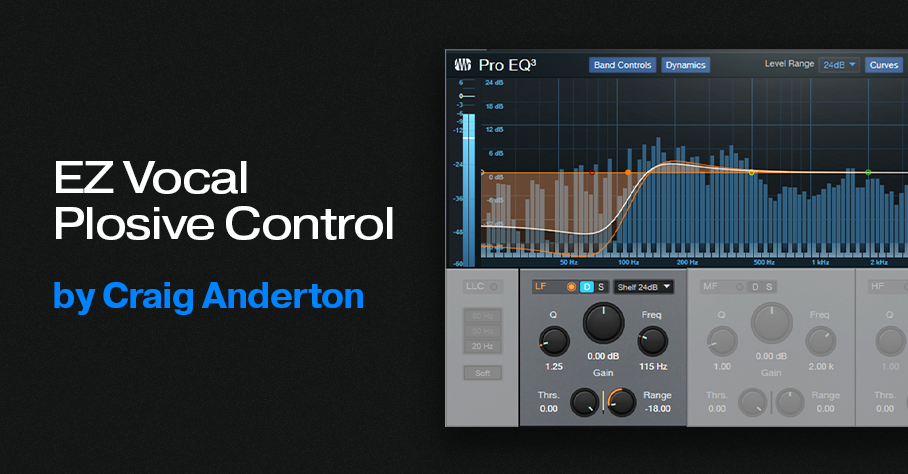
No matter how carefully you set up a mic’s pop filter, some pops are bound to get through the filter with vocalists who sing close to the mic. But you don’t need to redo or punch the vocal—let’s explore several ways to fix these problems in the mix.
Pro EQ3 dynamic EQ. Dynamic EQ is a fast, simple way to reduce pops (fig. 1):
1. Enable the low-frequency (LF) stage. Click the D button to reveal the dynamic EQ parameters.
2. Choose a 12 or 24 dB/octave low-frequency shelf.
3. Start with a substantial negative Range (e.g., ‑12 to ‑20).
4. Set Thrs. (threshold) to 0.00.
5. Loop the vocal section with the plosives. Adjust the low-shelf frequency so that the low-frequency attenuation affects only the plosives, not the voice’s usual warmth.
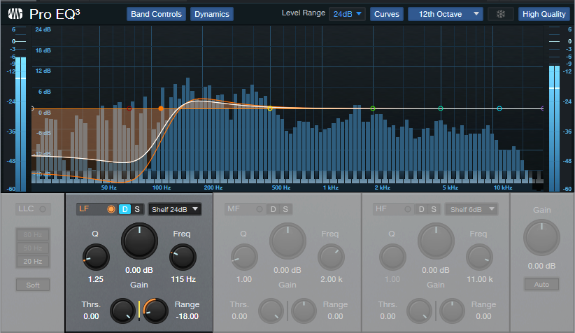
This technique also allows for a cool trick. Increase the Q slightly. When the plosives are being reduced, the increased Q adds a slight boost just above the shelf’s corner frequency. This gives some extra warmth to compensate for the lows being reduced.
Although this technique is simple to set up and works on an entire track, it may not be effective enough with super-nasty pops. The following methods are labor-intensive but can annihilate pretty much any plosive.
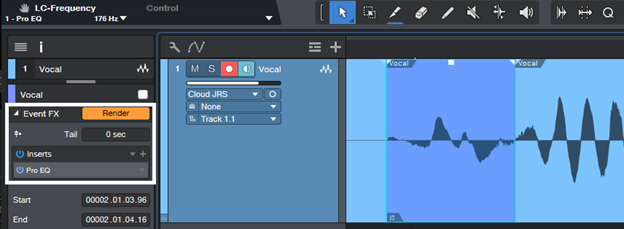
Split the Event before and after the pop, then insert Low Cut EQ as an Event FX. Roll off the low frequencies with the Event FX EQ (fig. 2). The only drawback is that if there are clicks when transitioning in or out of the isolated event, you’ll need to add crossfades or fades.
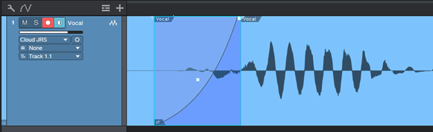
Split just before the pop, then fade in over the beginning (fig. 3). This reduces the level of the pop’s most prominent part—the beginning. For the best results, you need to find just the right split point prior to the pop, and carefully edit the fade shape.
For a solution that fixes plosives and sibilant (“ess”) sounds, check out The Vocal Repair Kit blog post. It’s also a tip in The Huge Book of Studio One Tips & Tricks v1.4 (see page 174).
15 Free “Analog” Cab IRs for Ampire
This week, I wanted to give y’all a little gift: 15 “analog cab” IRs that provide alternate User Cabinet sounds for Ampire. Just hit the download link at the bottom, and unzip.
If you’re not familiar with the concept of an analog cab, it’s about using EQ (not the usual digital convolution techniques) to model a miked cab’s response curve. This gives a different sonic character compared to digitally-generated cabs. (For more information, see Create Ampire Cabs with Pro EQ2.) An analogy would be that convolution creates a photograph of a cab, while analog techniques create a painting.
The 15 impulse responses (IRs) in the Ampire Analog Cab IRs folder were made by sending a one-sample impulse through EQ, and rendering the result. This process creates the WAV file you can then load into Ampire’s User Cabinet. The IRs include the following cab configurations: 1×8, 1×10, (4) 1×12, (3) 2×12, 4×10, and (5) 4×12.
How to Use Analog Cabs
- The simplest application is dragging an analog cab IR into Ampire’s User Cabinet image.
- To create cab stacks, insert different cabs in the User Cabinet’s three Mic slots. Vary their mix with the Mic Edit Controls.
- Layer two Ampires, one with a convolution-based cab impulse, the other with an analog cab impulse. This gives a “best of both worlds” sound.
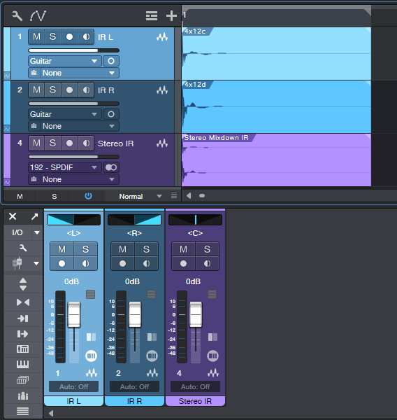
- Create stereo analog cabs that work with a single Ampire User Cabinet. Insert different analog cab IRs in two tracks, pan them oppositely, then export the mix (fig. 1 shows a typical setup). Drag the Event created by the export into Ampire’s User Cab. Note that the impulse response WAV files are very short—only 2,048 samples.
In any event, whether you go for individual impulses, layering, or creating stereo impulses, I think you’ll find that “analog” cab IRs extend Ampire’s sonic palette even further. And if you have any questions, or feedback on using analog cabs, feel free to take advantage of the Comments section!
Download the Ampire Analog Cab IRs.zip file below:
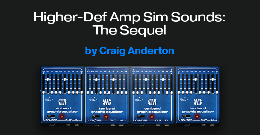
Higher-Def Amp Sim Sounds: The Sequel
Many of these tips have their genesis in asking “What if?” That question led to the Higher-Def Amp Sim Sounds blog post, which people seemed to like. But then I thought “What about taking this idea even further?” Much to my surprise, it could go further. This week’s tip, based on the Ampire High Density pack, is ideal for increasing the definition and articulation of high-gain and metal amp sims.
Fig. 1 shows the FX Chain (the download link is available at the end of this post). The Splitter is in Channel Split mode. If your guitar track is mono so it doesn’t have two channels, change the track mode to stereo and then bounce the Event to itself. This creates a dual mono track, which is optimum for this application.

With traditional multiband processing, each band represents a range of frequencies. Distorting a limited range of frequencies reduces intermodulation distortion. The result is a more defined, articulated sound quality.
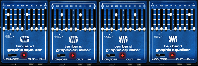
Fig. 1 implements a variation on multiband processing. It has four amps, but inserts Ampire’s Ten Band Graphic Equalizer before each amp. The graphic EQ sends two narrow frequency bands into each amp. Choosing frequency bands that are as far apart as possible reduces intermodulation distortion even further than standard multiband processing.
Referring to fig. 2, two bands in each graphic EQ are at +6 dB. The others are all at 0. Note how the various EQs offset the bands to different frequencies.
The Dual Pan plug-ins create a stereo image. With a traditional multiband setup, I tend to pan the low- and high-frequency bands to center, and spread the lower mids and upper mids in stereo. That doesn’t apply here, because there aren’t wide frequency ranges. Use whatever panning gives a stereo image you like.
A waveform is worth a thousand words, so check out the audio example. The first half is guitar going through Ampire’s German Metal amp sim. The second half uses this technique, with the same guitar track and amp sim settings. I think you’ll hear quite a difference.
Can This Be Taken Even Further?
Yes, it can—I also tried using eight splits. Because the Splitter module handles a maximum of five splits, I duplicated (complete) the track with the FX Chain, and fed both tracks with the same guitar part. The 31.2 Hz and 16 kHz bands aren’t particularly relevant, so I ignored those and fed one band from each EQ into an amp. As expected, this asks quite a bit of your CPU. Consider transforming the track to rendered audio (and preserving the realtime state, in case you need edits in the future).
However, I’m not convinced I liked the sound better. That level of definition seemed a little too clean for a metal amp sim. Sure, give it a try—but I feel the setup in this tip is the sweet spot of sound quality and convenience.
Download the FX Chain below!
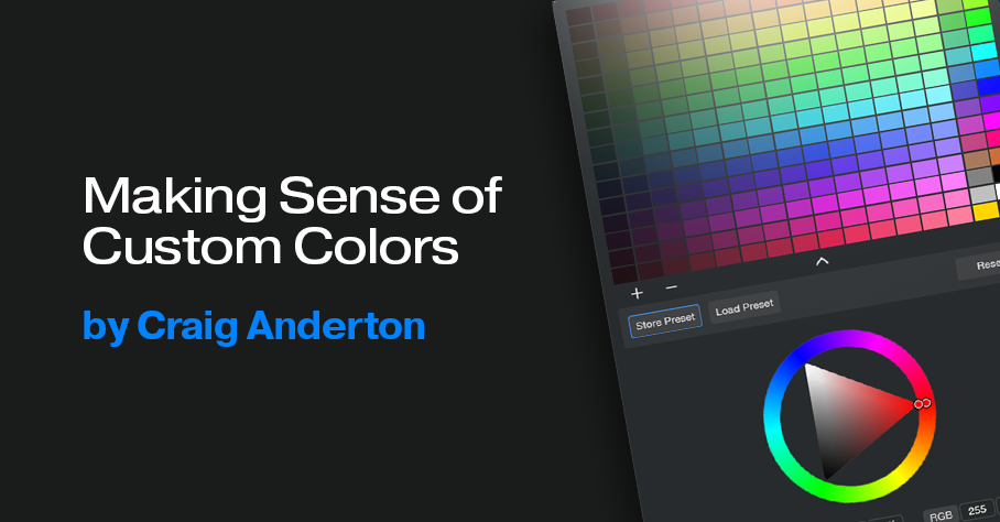
Making Sense of Custom Colors
Over four years ago, the blog post Colorization: It’s Not Just about Eye Candy covered the basics of using color. However, v6.1’s Custom Colors feature goes way beyond Studio One’s original way of handling colors.
The Help Viewer describes Custom Color operations, so we’ll concentrate on the process of customizing colors efficiently for your needs. For example, my main use for colors is to differentiate different track types (e.g., drums, synth, loops, voice, guitar, etc.). Then, changing the color’s brightness or saturation can indicate specific attributes within a track group, like whether a track is a lead part or background part, or whether a part is finished or needs further editing.
Opening the Custom Colors window and seeing all those colors may seem daunting. But as you’ll see, specifying the colors you want is not difficult.
What Are Hex, HSL, and RGB?
Electronic displays have three primary colors—red, green, and blue. Combining these produces other colors. For example, combining red and blue creates purple, while combining green and blue creates cyan. The three fields at the bottom of the expanded Custom Colors window (fig. 1) show the three main ways to define colors (left to right): Hex, HSL (Hue, Saturation, Lightness), and RGB (Red, Green, Blue). These are simply three different ways to express the same color.
RGB uses three sets of numbers, from 0 to 255, to express the values of Red, Green, and Blue. 255, 0, 0 would mean all red, no green, and no blue.
Hex strings together three sets of two hex digits. The first two digits indicate the amount of red, the second two the amount of green, and the final two the amount of blue.
HSL is arguably the most intuitive way to specific custom colors, so that’s the option selected in fig. 1.
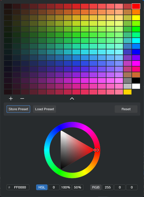
You can think of the spectrum of colors as a circle that starts at red, goes through the various colors, and ends up back at red. So, each color represents a certain number of degrees of rotation on that wheel. The number of degrees corresponds to the Hue (color), represented by the H in HSL. Each main color is 30 degrees apart along the wheel:
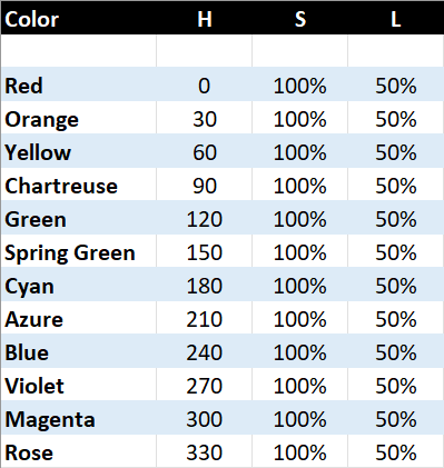
S represents the amount of saturation, from 0 to 100%. This defines the color’s vibrancy—with 100% saturation, the color is at its most vibrant. Pulling back on saturation mutes the color more. L is the luminance, which is basically brightness. Like saturation, the value goes from 0 to 100%. As you turn up luminance, the color becomes brighter until it washes out and becomes white. Turn luminance down, and the color becomes darker.
The Payoff of Custom Colors
Here’s why it’s useful to know the theory behind choosing colors. As mentioned at the beginning, I use two color variations for each group of tracks. For example, vocal tracks are green. I wanted bright green for lead vocals, and a more muted green for background vocals. For the bright green color, I created a custom color with HSL values of 120, 100%, and 50%. For the alternate color, I used the same values except for changing Saturation to 50%.
Fig. 2 shows the custom color parameter values used for the 12 main track groups. The right-most column in fig. 1 shows the main track group colors. The next column to the left shows the variation colors, which have 50% saturation. In the future, I’ll be adding more colors to the 12 original colors (for example, brown is the 13th color down from the top in fig. 1’s custom colors). Fortunately, the custom color feature lets you save and load presets.
The brain can parse images and colors more quickly than words, and this activity occurs mostly in the brain’s right hemisphere. This is the more intuitive, emotional hemisphere, as opposed to the left hemisphere that’s responsible for analytical functions like reading words. When you’re in the right hemisphere’s creative zone, you want to stay there—and v6.1’s track icons and custom colors help you do that.
But Wait…There’s More!
Don’t forget that Studio One also has overall appearance preferences at Options > Appearance. This is kind of like a “master volume control” for colors. If you increase contrast, the letters for track names, plugins, etc. really “pop.” For my custom colors, increasing the overall Luminance emphasizes the difference between the main track color and the variation track color.
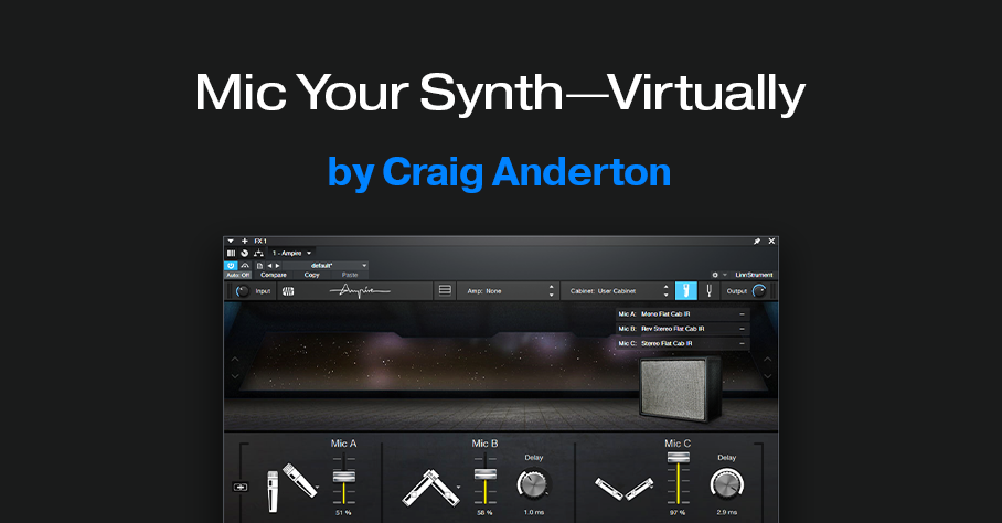
Mic Your Synth—Virtually
You can mic piano, drums, guitar, voice, and other acoustic sources…but you can’t mic a synth, unless you put it through a PA or guitar amp, and then mic that.
Or can you?
Studio One’s Ampire has mic modeling for its various cabs. However, a cab has its own frequency response, which doesn’t sound at all like miking an instrument—it sounds like miking a guitar amp. Sometimes, you want that sound with instruments other than guitar or bass. But usually, you don’t.
Ampire also has a User Cab for loading your own cab impulse responses. So, you could load a room’s impulse response instead, and set up Ampire’s mics. However, then you’re not miking an instrument, you’re miking the instrument in a room. What if you just want the sound of a miked instrument?
Here’s the solution, and I think you’ll be as surprised as I was after pulling up an FX bus fader with the sound of the virtual mics. Check out the audio example: the first half is a plain Mai Tai sound, the second half has the virtual miking. There are no effects, only Ampire’s mics. Of course, this is only one of many possibilities.
How It Works
The trick is to bypass the amp, and load a flat-response impulse into Ampire’s User Cab. Then, the audio doesn’t go through an amp or cab sound before hitting the mics. Simple, right?
The downloadable zip file (link at end) includes three flat-response IRs, each of which has its uses:
- Stereo (dual mono)
- Stereo with reversed left channel phase
- Stereo with reversed right channel phase
Ampire Prep
I prefer to set up Ampire in an FX bus, to enable blending the miked sound with the direct sound. However, using the miked sound by itself is viable. See which you prefer. Fig. 1 shows the Ampire settings used for the audio example.

To create the setup:
1. Insert Ampire in an FX bus.
2. Assign a Send to the FX bus from the instrument track you want to “mic.”
3. With Ampire, choose Amp: None and Cabinet: User Cabinet
4. Download and unzip the three impulse responses.
5. Click on the Mic Edit Controls button (the blue button in fig. 1), then click on the + sign next to Mic A. Navigate to your IR of choice, and load it. Or, simply drag the impulse into the Mic’s slot.
6. Similarly, load an IR into Mic B and Mic C. Note: There must be an IR loaded in Mic A, or no sound will pass through Ampire, even if IRs are loaded in Mic B and Mic C. I recommend loading an IR in each one.
7. Go down the fun rabbit hole of mic choices, levels, mic delays, and phase changes.
Extra Tips
- Using an IR with reversed phase for one of the mics can unbalance the stereo image. Compensate by adjusting the Panpot in the Send that goes to the FX Channel.
- In the FX Channel, spreading the stereo image with the panpot’s Binaural function is cool (pre-Studio One 6 owners can use the Binaural Pan plug-in). For the audio example, I turned up the Binaural Pan so the effect would be more dramatic if heard over laptop speakers.
- The audio example mixes the miked sound up quite a bit to get the point across, but subtle settings can add an interesting dimension to synthesized sounds.
- Preceding Ampire with an Analog Delay set for a very short delay (a few milliseconds) and no feedback can enhance the effect further.
- This isn’t just about synths—try this technique with other non-acoustic sounds, like analog drums.
Reminder!
If you bought a previous version of The Huge Book of Studio One Tips and Tricks, you can now download the free version 1.4 update (with 250 tips and 126 free presets) from the PreSonus shop.
Quick, Perfect S-Shaped Fades
First, some news: the free update to version 1.4 of The Huge Book of Studio One Tips and Tricks is finally available in the PreSonus Shop. If you purchased a previous version from PreSonus, simply download the eBook again, using the same credentials—you’ll automatically receive the latest version. Now for the tip…
What’s Cool About S-Shaped Fades, Anyway?
An S-shaped fade starts by fading slowly, accelerates to halfway through the fade, then slows down to do the final part of the fade. This provides a natural, smooth kind of fade that I prefer for most song fadeouts. Also, video tracks commonly use S-shaped fades. So, an S-shaped fade for the audio can match an S-shaped fade applied to the video.
Before version 5.5, the Project Page didn’t have automation or a gain envelope, so I wrote a tip on how to incorporate an S-shaped fade in a Song’s master level automation. Once the song had the fade, you could update the Mastering file to include the fade. But now that the Project Page can do automation and gain envelopes, you can apply that tip directly to Events in the Project Page as well as in the Song page.
However, compared to the technique this post covers, the previous method has one advantage and one disadvantage. The advantage is that it’s easy to customize the S-fade shape. The disadvantage is that it’s more time-consuming to get a perfect S-shape. So, here’s how to add a perfect S-shaped fade—quickly—with the Paint tool and its Parabolic option:
1. Add a Gain Envelope (right-click on an Event and check Gain Envelope). You can also apply this kind of fade to master level automation.
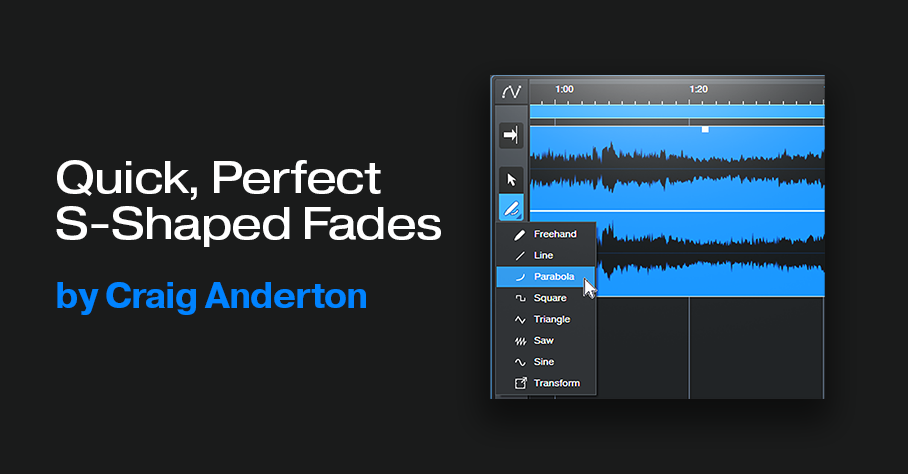
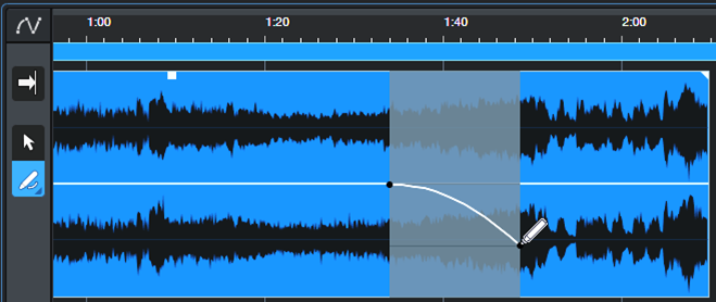
2. Choose the Parabola shape for the Pencil tool (fig. 1).
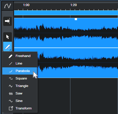
3. Click where you want the fade to begin. Drag right, and then down to where the fade’s midpoint should be (fig. 2).
4. Finally, click where you want the fade to end. Drag left, and then up to the fade’s midpoint (fig. 3).
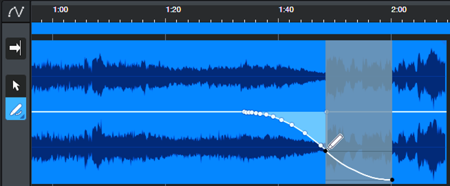
And now, you have your perfect S-shaped fadeout. Delete any nodes (if present) to the right of where the fade ends—and your work is done.