Category Archives: Uncategorized
How To Distribute Your Music with Studio One From Creation to Digital Streaming Platforms
If you’re a PreSonus user, you’re probably pretty hands-on in producing and recording your
music. Maybe you already know how to master spatial audio or are reading this blog to figure
out multitimbral instrumentation with guitar (no—seriously!).
These are vital skills for any independent musician. Distributing your music online can empower
you to take control of your music’s journey.
What is TuneCore?
If you’re reading this, your experience with digital distribution might be limited. That’s ok! Maybe
you’re only distributing to platforms like Soundcloud and Bandcamp. Perhaps you don’t even
know what a DSP is* and haven’t started your journey of sharing tracks with the public at large.
That’s where TuneCore comes in.
TuneCore is an independent artist development platform specializing in music distribution. Both
TuneCore and PreSonus are here to support you at every stage of your career, and distributing
your music online is one of the most critical aspects. This is why we partnered to build a
“creation-to-DSP” pipeline that Studio One and TuneCore users can benefit from.
However, it’s important to note that true support for artists begins with education. Understanding
the ins and outs of Music Distribution 101 is crucial for your success as an independent
musician. So, let’s dive in and demystify this essential aspect of your music career.
* DSP = digital service provider, i.e., Spotify, Apple Music, TIDAL, Amazon Music
How Digital Music Distribution Works
At its core, digital music distribution is simply the process of making your music available on
various online platforms or marketplaces.
Each platform or marketplace has its own technical and content guidelines, which must be
adhered to for music to be hosted. These can range from audio file format specifications to
correctly labeling an “explicit” song as such. We’ve broken them down in detail right here.
Tips to Distribute Your Music
If you don’t have time to read that, though (and who does?), save this cheat sheet for your
future use:
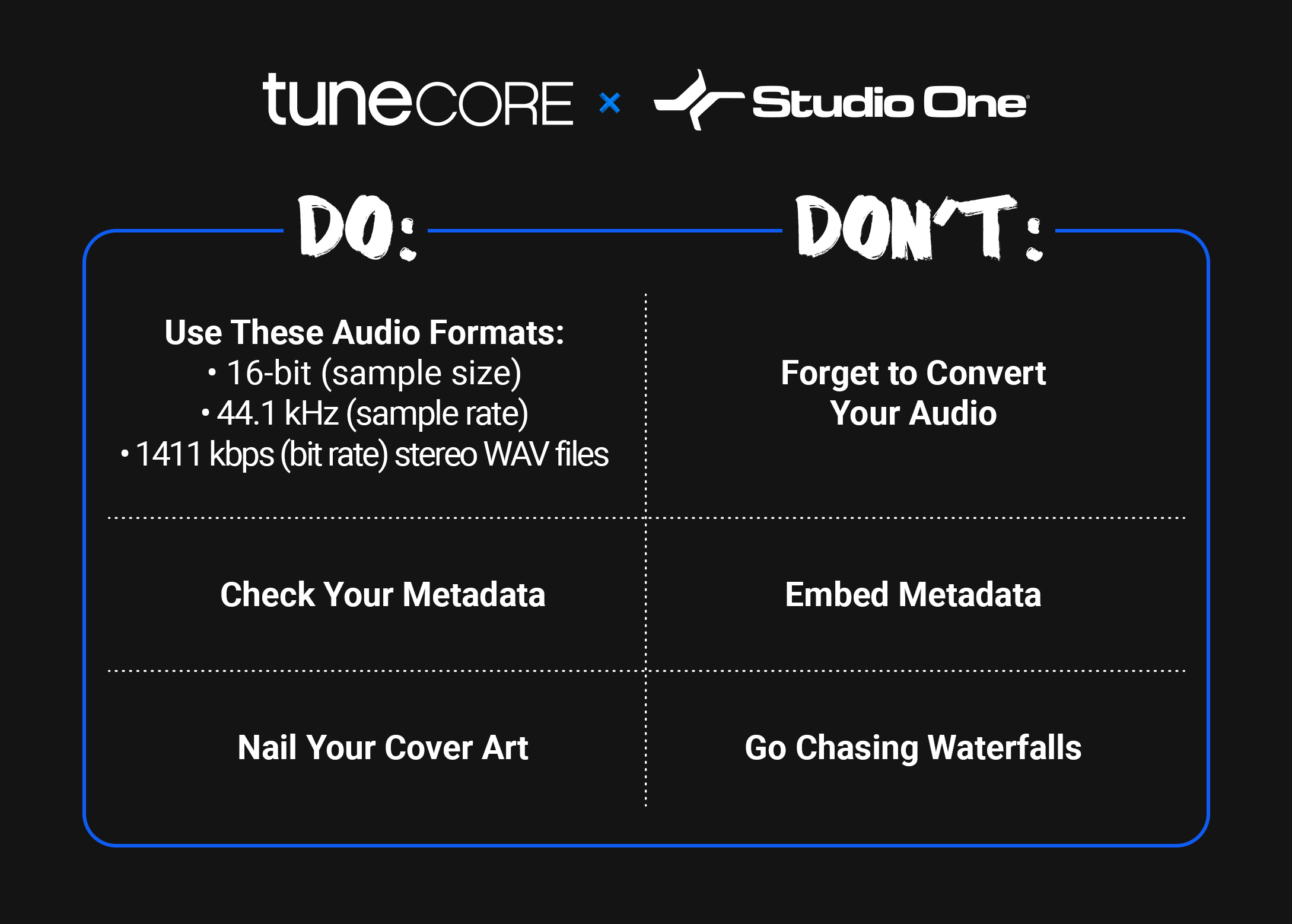
DO: Check Your Metadata
Painstakingly reviewing your metadata is one of the most vital components of the distribution
process. It’s also one of the most tedious. But it’s worth it.
From a music publishing perspective, metadata is king – and correctly inputting metadata
ensures that you get the most royalty matches possible to earn streams on DSPs like Spotify
and Apple Music, locations like bars and hotels, and so much more. We cannot stress this
enough: making sure your song’s metadata is accurate is of the utmost importance.
Similarly, your cover art is the face of your music, and it’s crucial to get it right.
Here are the five most important metadata components to check:
- IPI/CAE number – a unique identifier assigned to all songwriters and publishers who are
registered with a collection society (such as BMI or ASCAP - ISRC (And Release Info) – a unique,12-digit alphanumeric identifier that helps identify
the usage of your sound recordings and their underlying compositions (this helps you
collect publishing royalties) - ISWC – a unique, 10-character code identifying musical works that links to a song’s
recording (this helps you collect master royalties) - Alternative Titles & New Recordings – such as a live recording, another artist’s cover
version of your song, a remix, slowed or sped-up versions, etc. - Songwriters and Shares – Percent of Song Ownership
This can be overwhelming. The good news is that when you distribute through Studio One x
TuneCore, we’ll ask for and help you identify all this information. It won’t undergo TuneCore’s
review process until you’ve imputed it
DON’T: Embed Your Metadata
Given how vital metadata is to you getting paid for distributing your music, it’s understandably
vital that you don’t try to cut corners when inputting it.
Embedding is a form of cutting corners.
Having your metadata already attached to the track you’re uploading sounds convenient, but
let’s happily shatter that illusion. Digital stores don’t accept embedded files. Getting your music
to fans (and getting paid for it) means uploading tracks that pass a DSP’s content guidelines,
and embedding isn’t one of them.
Again, through Studio One’s integration with TuneCore, you’ll be able to enter all this metadata
yourself and ensure you’re good to go.
DO: Nail Your Cover Art
Regarding DSPs like Tidal or Amazon Music, audio isn’t the only component of a track with
content requirements.
Your cover art also needs to be in store-ready shape.
If you haven’t given this much thought, don’t sweat it. However, it’s important to note that not
meeting these requirements can lead to your music not being distributed on certain platforms.
Musicians are rightly more focused on their craft and a song’s audio fidelity than the technical
specters of the accompanying image.
Here are the components you MUST nail down to get your artwork cleared:
- Image Format: JPG or GIF
- Aspect Ratio: 1:1 (Perfect square)
- Resolution: At least 1600 x 1600 pixels in size
- Best quality RGB Color Mode (this includes black and white images)
- If you’re distributing your music to the Amazon On Demand store (for printing physical
CD covers), you need a resolution of 300 DPI.
Here’s what you CAN’T include:
- Words or phrases that don’t match the Artist Name or Song/Album Name
- Email addresses, URLs/websites, contact info (this includes social handles), or pricing
- Stickers from your artwork from a scanned copy of the physical CD
- Something that suggests the release format “CD, DVD, Digital Exclusive, the disc.”
- Cut off text or images
- An image that’s compressed into one corner with white space
- Names of digital stores or their logos
- Words that express temporality, like “new,” “latest single,” “limited edition,” or “exclusive.”
For even more information – like how to correctly attach cover art to your track – check out our
recent guide to cover art here.
DON’T: Go Chasing Waterfalls
This was a TLC joke.
We stand by it.
PreSonus x TuneCore
PreSonus made its name by making it easier than ever for musicians to achieve end-to-end
music creation. With Studio One – featuring Apple Spatial Audio and direct distribution through
TuneCore – that goal is a full-fledged reality.
As the above video illustrates, PreSonus x TuneCore users can get their music across the
proverbial finish line and into TuneCore’s capable hands for distribution without ever closing out
of Studio One.
The hardest part was learning the basics of music distribution. Now that you have, you can get
back to creating and releasing music.
We’ll handle the rest.
15 Free “Analog” Cab IRs for Ampire
This week, I wanted to give y’all a little gift: 15 “analog cab” IRs that provide alternate User Cabinet sounds for Ampire. Just hit the download link at the bottom, and unzip.
If you’re not familiar with the concept of an analog cab, it’s about using EQ (not the usual digital convolution techniques) to model a miked cab’s response curve. This gives a different sonic character compared to digitally-generated cabs. (For more information, see Create Ampire Cabs with Pro EQ2.) An analogy would be that convolution creates a photograph of a cab, while analog techniques create a painting.
The 15 impulse responses (IRs) in the Ampire Analog Cab IRs folder were made by sending a one-sample impulse through EQ, and rendering the result. This process creates the WAV file you can then load into Ampire’s User Cabinet. The IRs include the following cab configurations: 1×8, 1×10, (4) 1×12, (3) 2×12, 4×10, and (5) 4×12.
How to Use Analog Cabs
- The simplest application is dragging an analog cab IR into Ampire’s User Cabinet image.
- To create cab stacks, insert different cabs in the User Cabinet’s three Mic slots. Vary their mix with the Mic Edit Controls.
- Layer two Ampires, one with a convolution-based cab impulse, the other with an analog cab impulse. This gives a “best of both worlds” sound.
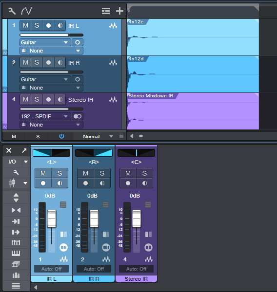
- Create stereo analog cabs that work with a single Ampire User Cabinet. Insert different analog cab IRs in two tracks, pan them oppositely, then export the mix (fig. 1 shows a typical setup). Drag the Event created by the export into Ampire’s User Cab. Note that the impulse response WAV files are very short—only 2,048 samples.
In any event, whether you go for individual impulses, layering, or creating stereo impulses, I think you’ll find that “analog” cab IRs extend Ampire’s sonic palette even further. And if you have any questions, or feedback on using analog cabs, feel free to take advantage of the Comments section!
Download the Ampire Analog Cab IRs.zip file below:
Higher-Def Amp Sim Sounds: The Sequel
Many of these tips have their genesis in asking “What if?” That question led to the Higher-Def Amp Sim Sounds blog post, which people seemed to like. But then I thought “What about taking this idea even further?” Much to my surprise, it could go further. This week’s tip, based on the Ampire High Density pack, is ideal for increasing the definition and articulation of high-gain and metal amp sims.
Fig. 1 shows the FX Chain (the download link is available at the end of this post). The Splitter is in Channel Split mode. If your guitar track is mono so it doesn’t have two channels, change the track mode to stereo and then bounce the Event to itself. This creates a dual mono track, which is optimum for this application.

With traditional multiband processing, each band represents a range of frequencies. Distorting a limited range of frequencies reduces intermodulation distortion. The result is a more defined, articulated sound quality.
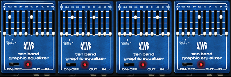
Fig. 1 implements a variation on multiband processing. It has four amps, but inserts Ampire’s Ten Band Graphic Equalizer before each amp. The graphic EQ sends two narrow frequency bands into each amp. Choosing frequency bands that are as far apart as possible reduces intermodulation distortion even further than standard multiband processing.
Referring to fig. 2, two bands in each graphic EQ are at +6 dB. The others are all at 0. Note how the various EQs offset the bands to different frequencies.
The Dual Pan plug-ins create a stereo image. With a traditional multiband setup, I tend to pan the low- and high-frequency bands to center, and spread the lower mids and upper mids in stereo. That doesn’t apply here, because there aren’t wide frequency ranges. Use whatever panning gives a stereo image you like.
A waveform is worth a thousand words, so check out the audio example. The first half is guitar going through Ampire’s German Metal amp sim. The second half uses this technique, with the same guitar track and amp sim settings. I think you’ll hear quite a difference.
Can This Be Taken Even Further?
Yes, it can—I also tried using eight splits. Because the Splitter module handles a maximum of five splits, I duplicated (complete) the track with the FX Chain, and fed both tracks with the same guitar part. The 31.2 Hz and 16 kHz bands aren’t particularly relevant, so I ignored those and fed one band from each EQ into an amp. As expected, this asks quite a bit of your CPU. Consider transforming the track to rendered audio (and preserving the realtime state, in case you need edits in the future).
However, I’m not convinced I liked the sound better. That level of definition seemed a little too clean for a metal amp sim. Sure, give it a try—but I feel the setup in this tip is the sweet spot of sound quality and convenience.
Download the FX Chain below!
Making Sense of Custom Colors
Over four years ago, the blog post Colorization: It’s Not Just about Eye Candy covered the basics of using color. However, v6.1’s Custom Colors feature goes way beyond Studio One’s original way of handling colors.
The Help Viewer describes Custom Color operations, so we’ll concentrate on the process of customizing colors efficiently for your needs. For example, my main use for colors is to differentiate different track types (e.g., drums, synth, loops, voice, guitar, etc.). Then, changing the color’s brightness or saturation can indicate specific attributes within a track group, like whether a track is a lead part or background part, or whether a part is finished or needs further editing.
Opening the Custom Colors window and seeing all those colors may seem daunting. But as you’ll see, specifying the colors you want is not difficult.
What Are Hex, HSL, and RGB?
Electronic displays have three primary colors—red, green, and blue. Combining these produces other colors. For example, combining red and blue creates purple, while combining green and blue creates cyan. The three fields at the bottom of the expanded Custom Colors window (fig. 1) show the three main ways to define colors (left to right): Hex, HSL (Hue, Saturation, Lightness), and RGB (Red, Green, Blue). These are simply three different ways to express the same color.
RGB uses three sets of numbers, from 0 to 255, to express the values of Red, Green, and Blue. 255, 0, 0 would mean all red, no green, and no blue.
Hex strings together three sets of two hex digits. The first two digits indicate the amount of red, the second two the amount of green, and the final two the amount of blue.
HSL is arguably the most intuitive way to specific custom colors, so that’s the option selected in fig. 1.
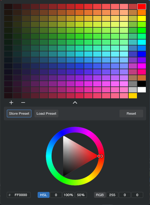
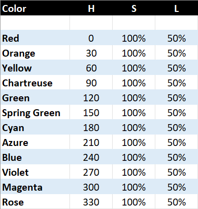
You can think of the spectrum of colors as a circle that starts at red, goes through the various colors, and ends up back at red. So, each color represents a certain number of degrees of rotation on that wheel. The number of degrees corresponds to the Hue (color), represented by the H in HSL. Each main color is 30 degrees apart along the wheel:
S represents the amount of saturation, from 0 to 100%. This defines the color’s vibrancy—with 100% saturation, the color is at its most vibrant. Pulling back on saturation mutes the color more. L is the luminance, which is basically brightness. Like saturation, the value goes from 0 to 100%. As you turn up luminance, the color becomes brighter until it washes out and becomes white. Turn luminance down, and the color becomes darker.
The Payoff of Custom Colors
Here’s why it’s useful to know the theory behind choosing colors. As mentioned at the beginning, I use two color variations for each group of tracks. For example, vocal tracks are green. I wanted bright green for lead vocals, and a more muted green for background vocals. For the bright green color, I created a custom color with HSL values of 120, 100%, and 50%. For the alternate color, I used the same values except for changing Saturation to 50%.
Fig. 2 shows the custom color parameter values used for the 12 main track groups. The right-most column in fig. 1 shows the main track group colors. The next column to the left shows the variation colors, which have 50% saturation. In the future, I’ll be adding more colors to the 12 original colors (for example, brown is the 13th color down from the top in fig. 1’s custom colors). Fortunately, the custom color feature lets you save and load presets.
The brain can parse images and colors more quickly than words, and this activity occurs mostly in the brain’s right hemisphere. This is the more intuitive, emotional hemisphere, as opposed to the left hemisphere that’s responsible for analytical functions like reading words. When you’re in the right hemisphere’s creative zone, you want to stay there—and v6.1’s track icons and custom colors help you do that.
But Wait…There’s More!
Don’t forget that Studio One also has overall appearance preferences at Options > Appearance. This is kind of like a “master volume control” for colors. If you increase contrast, the letters for track names, plugins, etc. really “pop.” For my custom colors, increasing the overall Luminance emphasizes the difference between the main track color and the variation track color.
How to “Focus” Effects
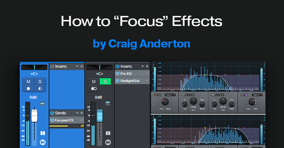
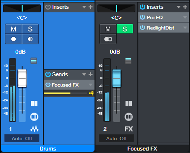
There’s nothing new about using an FX Channel to add an effect in parallel to a main track. But we can make effects even more effective by “tuning” them, to provide more focus.
This process works by inserting a Pro EQ3 before an FX Channel effect or effects (fig. 1). Then, use the EQ’s Low Cut and High Cut filters to tune a specific frequency range that feeds the effect. For example, I’ve mentioned restricting high and low frequencies prior to feeding amp sims, but we can use this focusing technique with any processor.
There are several reasons for placing the Pro EQ3 before the effect. With saturation effects, this reduces the possibility of intermodulation distortion. With other effects, reducing the level of unneeded frequencies opens up more headroom in the effect itself. Finally, with effects that respond to dynamics (autofilter, compressor, etc.), you won’t have frequencies you don’t want pushing the frequencies you do want over the processor’s threshold.
Here are some specific examples to help get your creative juices flowing.
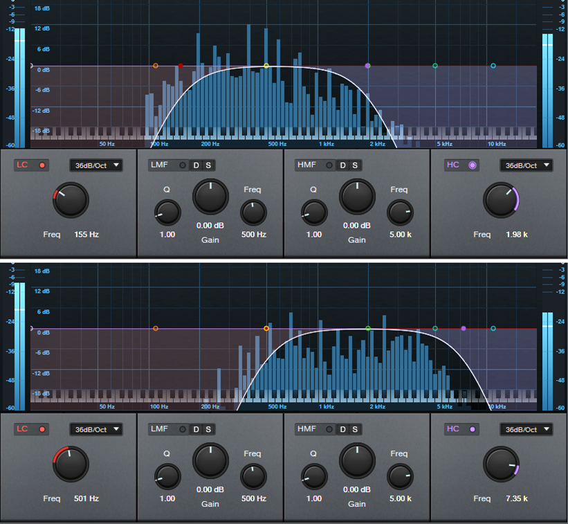
Distortion or Saturation with Drums
The audio example plays four measures of drums going into the RedlightDist, with no focus. The next four measures focus on the high frequencies. This gives an aggressive “snap” to the snare. The next four measures focus on the low frequencies, to push the kick forward.
Fig. 2 shows the tunings for the high- and low-frequency focus.

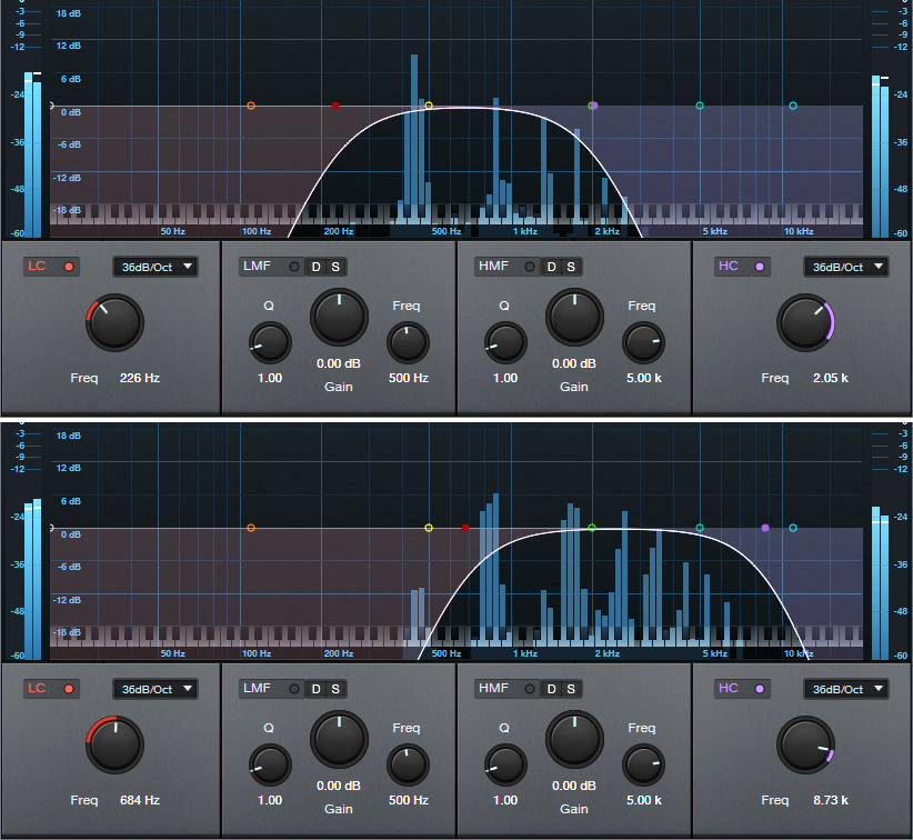
Reverb with Guitar
The audio example plays four measures of midrange-frequency focus feeding reverb, then four measures using a high-frequency focus. Focusing is helpful with longer reverb times, because there are fewer frequencies to interfere with the main sound.
Fig. 3 shows the tunings for the midrange- and high-frequency focus filters.
Delay with Synth Solo
For our last example, the first five measures are synth with no focus. The next five measures focus on the lower frequencies. The difference is subtle, but it “tucks away” the reverb behind the solo line. The final five measures focus on the high frequencies, for a more distant echo vibe.
Fig. 4 shows the tunings for the midrange- and high-frequency focus filters.
These are just a few possibilities—another favorite of mine is sending focused frequencies to a chorus, so that the chorus effect doesn’t overwhelm an instrument. Expanders also lend themselves to this approach, as does saturation with bass and electric pianos.
Perhaps most importantly, focusing the effects can give a less cluttered mix. Even tracks with heavy processing can stand out, and sound well-defined.
Better Autofilter Control

The March 2020 blog post, Taming the Wild Autofilter, never appeared in any of The Huge Book of Studio One Tips & Tricks eBook updates. This is because the tip worked in Studio One 4, but not in Studio One 5. However, Studio One 6 has brought the Autofilter back to its former glory (and then some). Even better, we can now take advantage of FX Bus sends and dynamic EQ. So, this tip is a complete redo of the original blog post. (Compared to a similar tip in eBook version 1.4, this version replaces the Channel Strip with the Pro EQ3 for additional flexibility.)
The reason for coming up with this technique was that although I’d used the Autofilter for various applications, I couldn’t get it to work quite right for its intended application with guitar or bass. Covering the right filter cutoff range was a problem—for example, it wouldn’t go high enough if I hit the strings hard, but if I compensated for that by turning up the filter cutoff, then the cutoff wouldn’t go low enough with softer picking. Furthermore, the responsiveness varied dramatically, depending on whether I was playing high on the neck, or hitting low notes on the low E and A strings. This tip solves these issues.
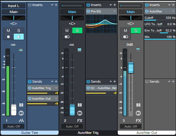
The guitar track’s audio uses pre-fader sends to go to two FX Buses (fig. 1). The Autofilter Out FX Bus produces the audio output. The Autofilter Trig FX bus processes the audio going to the Autofilter’s sidechain. By processing the Guitar track’s send to the sidechain, we can make the Autofilter respond however we want. Furthermore, if needed, you can feed a low-level signal from the Guitar track’s pre-fader send into the Autofilter, to avoid distortion with high-resonance settings. This is possible because the Autofilter Trig bus—which you don’t need to hear, and can be any level you want—controls the Autofilter’s action.
Perhaps best of all, this also means the Autofilter no longer depends on having an input signal with varying dynamics. You can insert an amp sim, overdrive, compressor, or anything else that restricts dynamic range in front of the Autofilter. The Autofilter will still respond to the original Guitar track’s dynamics, as processed by the dynamic EQ.
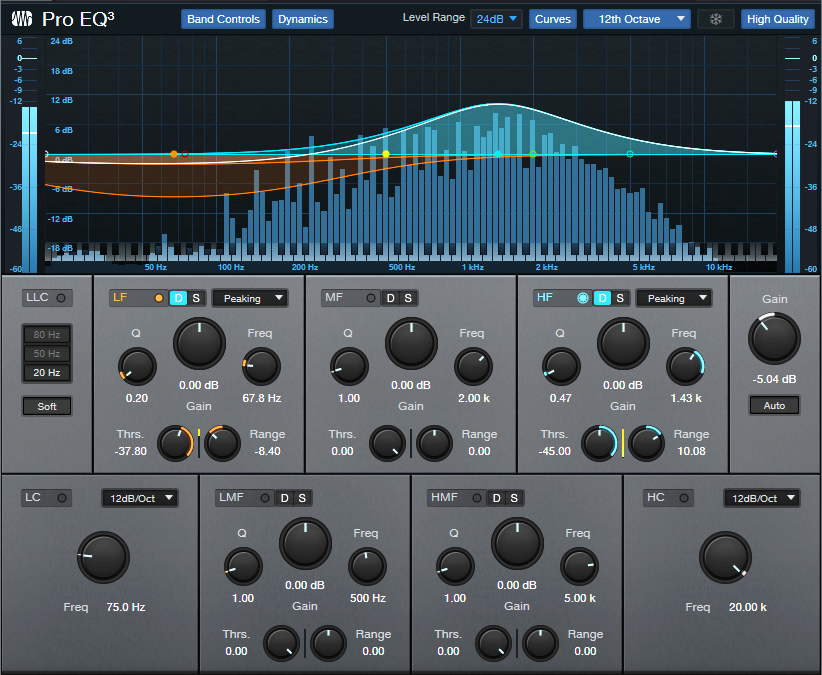
The Pro EQ3 (fig. 2) conditions the send to make the Autofilter happy. The dynamic EQ attenuates lower frequencies that exceed the Threshold, but amplifies higher frequencies that exceed the Threshold. So, the Autofilter’s response to the higher-output, lower strings can be consistent with the upper strings.
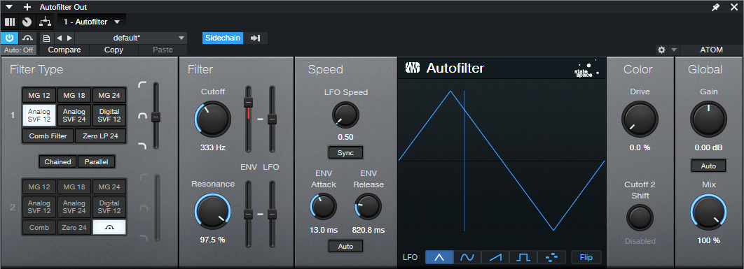
The Autofilter (fig. 3) sets the LFO Cutoff Modulation to 0, because I wanted only the envelope to affect the filter. The settings for the Autofilter and Pro EQ3 interact with each other, as well as with the guitar and pickups. In this case, I used a Telecaster with a single-coil treble pickup. For humbucking pickups, you may need to attenuate the low frequencies more.
Like Autofilters in general, it takes some experimenting to dial in the ideal settings for your playing style, strings, pickups, musical genre, and so on. However, the big advantage of this approach is that once you find the ideal settings, the response will be less critical, more consistent, and more forgiving of big dynamic changes in your playing.
And here’s a final tip: Processing the signal going to the Autofilter’s sidechain has much potential. Try using Analog Delay, X-Trem, and other effects. Also, although the original Guitar track and Autofilter Trig faders are shown at 0, no law says they have to be. Feel free to mix in some of the original guitar sound, and/or the equalized Autofilter Trig bus audio.
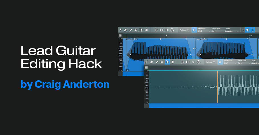
Lead Guitar Editing Hack
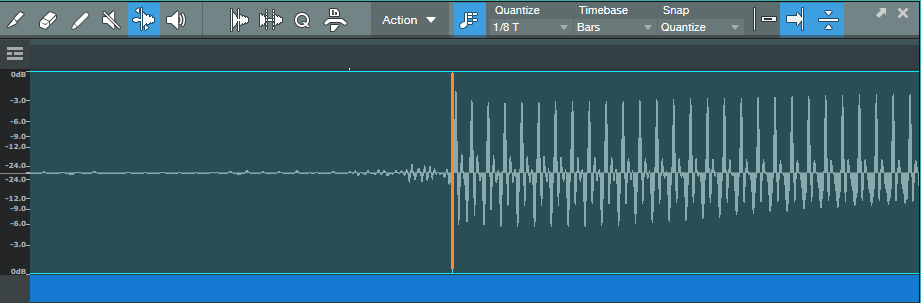
High-gain distortion is great for lead guitar sustain and tone, but it also brings up that “splat” of pick noise at the note’s beginning. Sometimes, you want the gritty, dirty feel it adds. But it can be a distraction when your goal is a gentler, more lyrical tone that still retains the sound of heavy distortion.
This technique gives the best of both worlds for single-note leads, and is particularly effective with full mixes where the lead guitar has a lot of echo. Normally the echo will repeat the pick noise, so reducing it reduces clutter, and gives more clarity to the mix.
1. Open the lead part in the Edit window.
2. Choose Action, and under the Audio Bend tab, select Detect Transients.
3. Zoom in to verify there’s a Bend Marker at the beginning of each note’s first peak (fig. 1). If you need to add a Bend Marker, click at the note’s beginning using the Bend tool. To move a Bend Marker for more precise placement, hold Alt/Opt while clicking on the marker with the Bend tool, and drag.
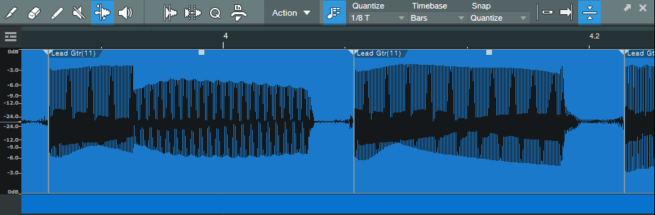
4. Choose Action, and under the Audio Bend tab, select Split at Bend Markers. Now, each note is its own Event (fig. 2).

5. Make sure all the notes are selected (fig. 3). The next steps show any needed edits being made to one Event. However, because all the notes are selected, any edit affects all notes equally. To show the edits in more detail, the following steps zoom in on two notes.
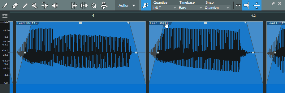
6. Trim the note ends to remove some of the pre-note “dirt” (fig. 4).

7. Add a fade-in and fade-out (fig. 5). This doesn’t have to be exact, because you’ll optimize the times in step 9.
8. There’s a gap between notes, so time-stretch the end of the note to cover the gap. Alt/Opt+click on the end of a note, and drag to the right until the note end is up against the beginning of the next note (fig. 6).
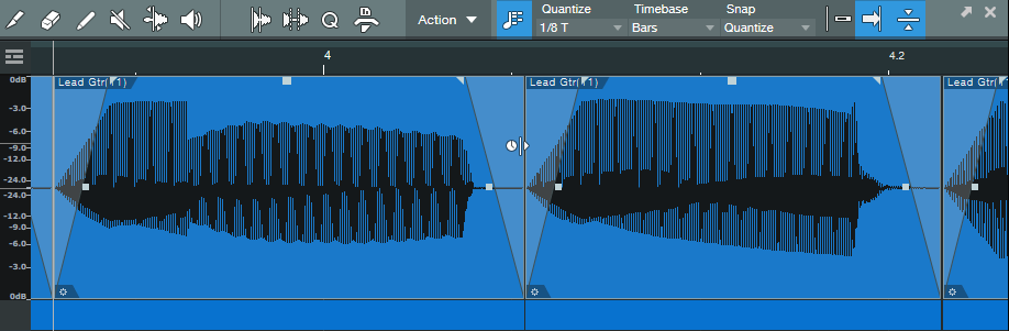
9. That may seem like a lot of work, but once you’ve defined the bend markers, having to edit only one note to edit all the notes speeds the process.
Start playback with all the notes still selected, listen, and vary the fade times. Also experiment with the curve shape. A concave curve can work well with attacks. I often try for the minimum amount of attack and decay that gives the desired result, but not always—when taken to extremes, being able to shape notes enables options that sound almost like a synthesizer.
The audio example shows how this tweak affects a single-note lead. The first part is as recorded, the second part uses this tip.
How to Use Virtual Synths as Signal Processors
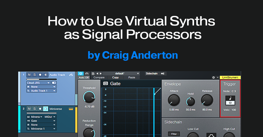
Some virtual instruments can accept external audio inputs. This lets you process audio through the synthesizer’s various modules like filters, VCAs, effects, and so on. Essentially, the synthesizer becomes an effects processor. To accommodate this, Version 6 introduced a sidechain audio input for virtual instruments.
Not all instruments have this capability. I’ve tested the audio sidechain input successfully with Cherry Audio’s CA2600, Miniverse, PS-30, Rackmode Vocoder, and Voltage Modular. Arturia’s Vocoder V also works. I’d really appreciate any notes in the Comments section about other instruments that work with this feature.
Is My Virtual Instrument Compatible?
Insert the synth, and click on the sidechain symbol in its header. If you see a box with Send and Output options (fig. 1), you can feed audio into the synthesizer. Check the box for either a Send from a track (pre- or post-fader), or the track output.

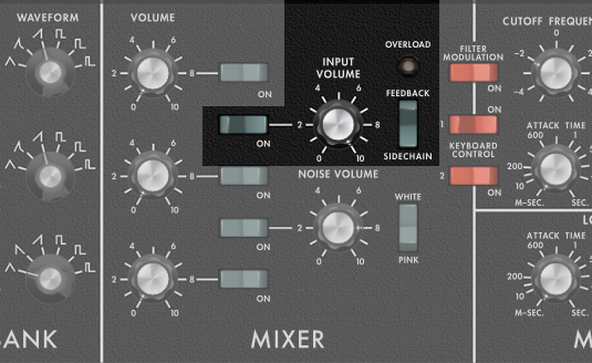
You’ll probably need to enable the virtual instrument’s external audio input. Fig. 2 shows how to do this with Cherry Audio’s Miniverse, which emulates how the Minimoog accepted external inputs:
- Set the Input’s Mixer switch to on.
- Turn up the Input volume.
- The Miniverse can feed the external input from its own output to obtain feedback, or from the Sidechain. For this application, choose Sidechain.
Studio One Setup
Fig. 3 shows the track layout for Studio One. Ignore the Gate for now, we’ll cover that shortly.
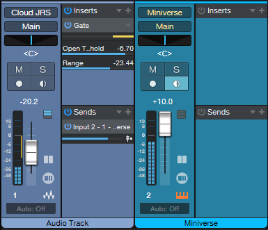
I chose a post-fader Send from the audio track, not the track output, to drive the synth. This is because I wanted to be able to mix parallel tracks—the audio providing the input, and the audio processed by the synthesizer.
Using the Gate
You won’t hear anything from the synth unless you trigger the VCA to let the external audio signal through. You can play a keyboard to trigger the synth for specific sections of the audio track, but the Gate can provide automatic triggering (fig. 4).
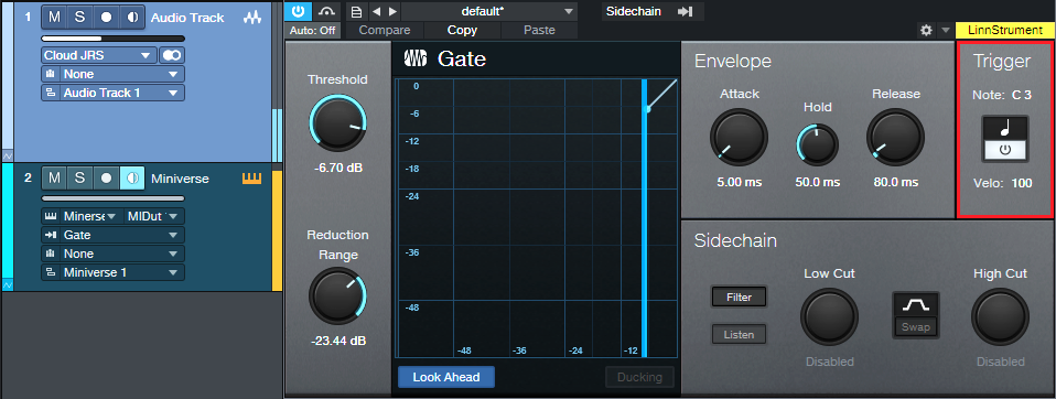
With Triggering enabled, the Gate produces a MIDI note trigger every time it opens. So, Insert the Gate in the audio track, and set the Instrument track’s MIDI input to Gate. Now, the audio will trigger the synth. Adjust the Gate Threshold for the most reliable triggering. This is particularly useful with instruments that have attacks, like drums, guitar, piano, etc.
Import JPG/PNG Files into the Video Track
This builds on last week’s tip about splitting and navigating within the Video Track, because one of the main reasons for creating splits is to import additional material. Although the Video Track can accept common video file formats, sometimes you’ll need to import static JPG or PNG images. These could be a band logo, screen shots for a tutorial video, a slide with your web site and contact information, photos from a smartphone, public domain images, etc. To bring them into the video track, you need to convert them into a compatible format, like MP4.
Many online sites offer to “convert JPEG to MP4 for free!” However, I’m skeptical of those kinds of sites. Fortunately, modern Mac and Windows operating systems include tools that can do any needed conversion.
Converting with the Mac
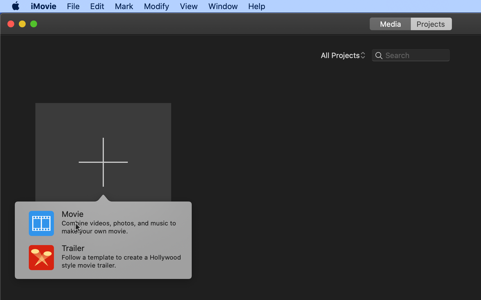
1. Open iMovie, click on Create New, and then choose Movie.
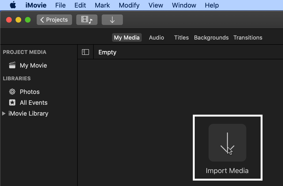
2. Click on Import Media. Navigate to the location of the image you want to convert, and open it in iMovie.
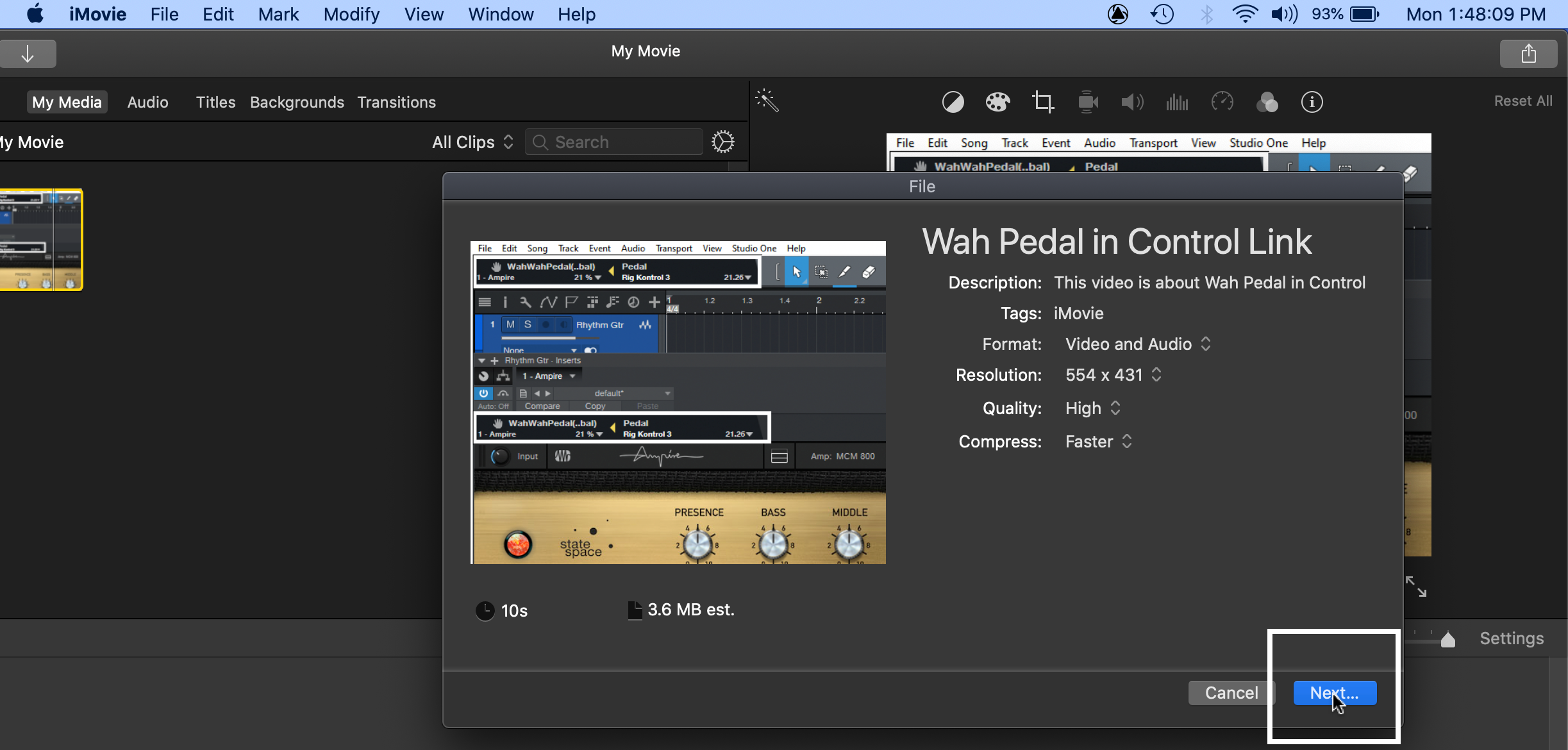
3. Choose File > Share > File.
4. In the window that opens, click Next…
5. Navigate to where you want to save the file, and click on Save. You now have an MP4 file.
If you need a longer video than the default 3 seconds, drag more copies of the file to the timeline before saving. Or, drag the file into Studio One multiple times.
Converting with Windows
1. Open Video Editor (it’s not necessary to install Clipchamp). Click on New Video, and name it.
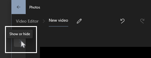
2. Click on the nearly invisible Project Library button.
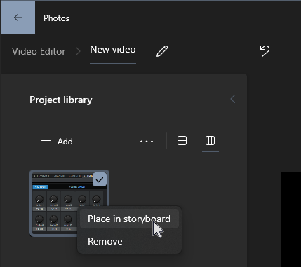
3. Drag the image you want to convert into the Library. Then right-click on the image, and choose Place in Storyboard. The default length is 3 seconds. If it needs to be longer, select Place in Storyboard again. Or, drag the finished file into Studio One multiple times.
4. Click on Finish video (in the upper right), then click on Export.
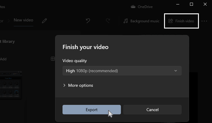
5. Name the file, navigate to where you want to save it, then click on Export. Done! Your image is now an MP4 video you can insert into Studio One.
Dual-ing Vocoders
What’s better than one vocoder? Two vocoders, of course 😊. This tip is more about a technique than an application, although we’ll cover an application to illustrate the technique. But the main goal is to inspire you to try stereo vocoding and come up with your own applications, so there are additional tips at the end.
Long-time blog readers may have noticed my fascination with fusing melodic and percussive components. The easiest way to do this is to have a drum track (or reverb, pink noise, hand percussion, whatever) follow the Chord Track via Harmonic Editing. Although this tip takes that concept further, it’s about more than just percussion. Inserting a Splitter in an FX Chain, and following it with two vocoders, opens sonic options you can’t obtain any other way.
The FX Chain and Track Layout
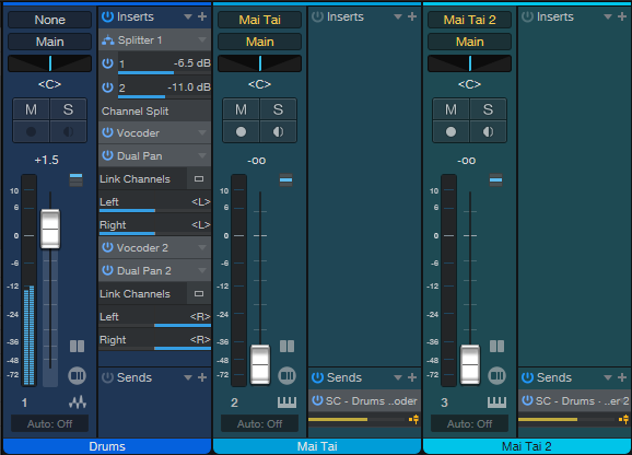
Fig. 1 shows the stereo vocoder FX Chain. This technique will also work with Artist. However, it requires three tracks:
- One with the modulator signal
- Two tracks whose inputs are set to the modulator track output. The vocoders go into these tracks.
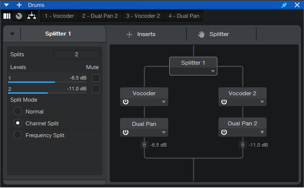
This application uses stereo drums, so the Splitter mode is Channel Split. The Dual Pan modules at the vocoder outputs provide stereo imaging. I typically pan one vocoder full left and the other full right, but sometimes I’ll weight them more to center, or to one side of the stereo field.
Fig. 2 shows the track layout. Each Mai Tai instrument track has a Send. These feed the sidechains for the two vocoders to provide the carrier audio. Although the Mai Tai faders are at minimum, mixing in some instrument sound provides yet another character.
Applications
This brief audio example adds a melodic component to drums. The two Mai Tai MIDI tracks are offset by an octave.
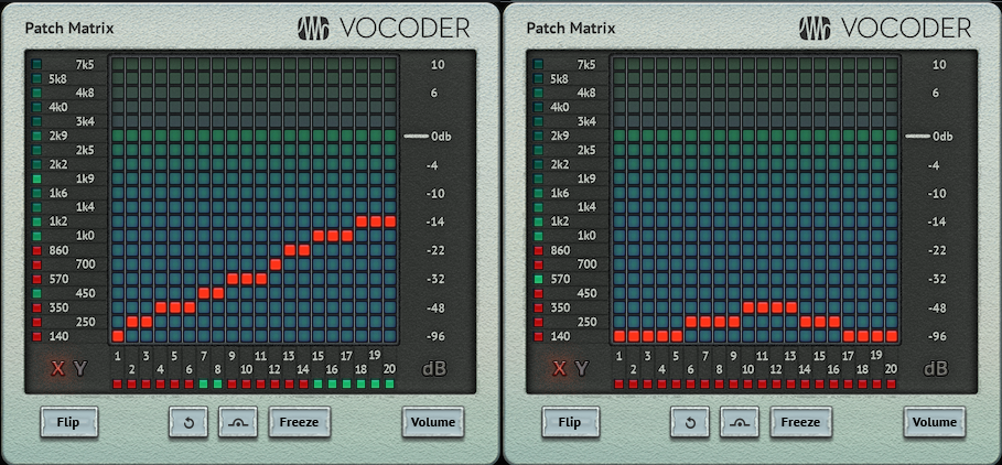
Fig. 3 shows the vocoder patch matrices. These particular settings are of no real consequence, they just emphasize that using different patch matrix settings for the left and right channel vocoders can have a major impact on the sound.
As to other applications:
- Depending on the source, using the Splitter’s Normal and Frequency Splits can work well.
- With anything percussive, try a Send from the Modulator track to a bus with Analog Delay, set to a rhythmic value.
- The vocoder Mix controls are the best way to introduce some of the modulator signal in with the “vocoded” signal.
- Adding Noise for Unvoiced Replacement fills out the sound in interesting ways. Turning up the modulator Attack and Release allows effects that are somewhat like mixing in a shaker or other hand percussion instrument.
- Try using audio as a carrier for one vocoder, the internal carrier for the other vocoder, and pan both vocoders to center.
- Using drums to modulate bass, and adding this as an almost subliminal effect to the main bass instrument sound, locks the bass tightly to a sense of rhythm.