Conventional wisdom says that compared to compression, limiting is a less sophisticated type of dynamics control whose main use is to restrict dynamic range to prevent issues like overloading of subsequent stages. However, I sometimes prefer limiting with particular signal sources. For example:

• For mixed drum loops, limiting can bring up the room sound without having an overly negative effect on the drum attacks.
• With vocals, I often use a limiter prior to compression. By doing the “heavy lifting” of limiting peaks, the subsequent compressor doesn’t have to work so hard, and can do what it does best.
• When used with slightly detuned synth patches, limiting preserves the characteristic flanging/chorusing-like sound, while keeping the occasional peaks under control.
• Limiting is useful when following synth sounds with resonant filters, or with instruments going through wah or autofilter effects

THE E-Z LIMITER

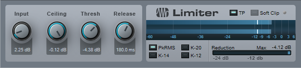
Some limiters (especially some vintage types) are easy to use, almost by definition: One control sets the amount of limiting, and another sets the output level. But Studio One’s limiter has four main controls—Input, Ceiling, Threshold, and Release—and the first three interact.

If the Studio One Limiter looked like Fig. 1, it would still take care of most of your needs. In fact, many vintage limiters don’t go much beyond this in terms of functionality.

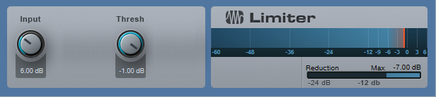
Figure 1: If Studio One’s Limiter had an “Easy Mode” button, the result would look something like this.

To do basic limiting:

1. Load the Limiter’s default preset.
2. Turn up the input for the desired limiting effect. The Reduction meter shows the amount of gain reduction needed to keep the output at the level set by the Threshold control (in this case, -1.00 dB). For example, if the input signal peaks at 0 dB and you turn up the Input control to 6 dB, the Limiter will apply 7 dB of gain reduction to keep the Limiter output at -1.00.

Note that in this particular limiting application, the Threshold also determines the maximum output level.

THE SOFT CLIP BUTTON

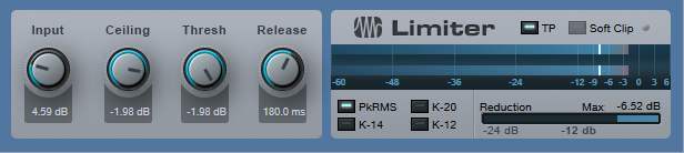
When you set Threshold to a specific value, like 0.00 dB, then no matter how much you turn up the Limiter’s Input control, the output level won’t exceed 0.00 dB. However, you have two options of how to do this.

• With Soft Clip off, gain reduction alone prevents the waveform from exceeding the ceiling.
• With Soft Clip on, clipping the peaks supplements the gain reduction process to keep the waveform from exceeding the ceiling (Fig. 2).

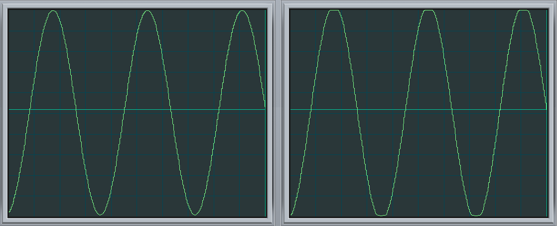
Figure 2: The left screen shot shows the waveform with the input 6 dB above the Threshold, and Soft Clip off. The right screen shows the same waveform and levels, but with Soft Clip turned on. Note how the waveform peak is flattened somewhat due to the mild saturation.

While it may sound crazy to want to introduce distortion, in many cases you’ll find you won’t hear the effects of saturation, and you’ll have a hotter output signal.

ENTER THE CEILING

There are two main ways to set the maximum output level:

• With the Threshold set to 0.00, set the maximum output level with the Ceiling control (from 0 to -12 dB).
• With the Ceiling set to 0.00, set the maximum output level with the Threshold control (from 0 to -12 Db).

It’s also possible to set maximum output levels below -12.00 dB. Turn either the Ceiling or Threshold control all the way counter-clockwise to -12.00 dB, then turn down the other control to lower the maximum output level. With both controls fully counter-clockwise, the maximum output level can be as low as -24 dB.

SMOOTHING THE TRANSITION INTO LIMITING

Setting the Ceiling lower than the Threshold is a special case, which allows smoothing the transition into limiting somewhat. Under this condition, the Limiter applies soft-knee compression as the input transitions from below the threshold level to above it.

For example, suppose the Ceiling is 0.00 dB and the Threshold is -6.00 dB. As you turn up the input, you would expect that the output would be the same as the input until the input reaches around -6 dB, at which point the output would be clamped to that level. However in this case, soft-knee compression starts occurring a few dB below -6.00 dB, and the actual limiting to -6.00 dB doesn’t occur until the input is a few dB above -6.00 dB.

The tradeoff for smoothing this transition somewhat is that the Threshold needs to be set below 0.00. In this example, the maximum output is -6.00 dB. If you want to bring it up to 0.00 dB, then you’ll need to add makeup gain using Mixtool module.

Studio One’s Limiter is a highly versatile signal processor, so don’t automatically ignore it in favor of the Compressor or Multiband Dynamics—with some audio material, it could be exactly what you need.

Some instruments, when compressed, lack “sparkle” if the stronger, lower frequencies compress high frequencies as well as lower ones. This is a common problem with guitar, but there’s a solution: the Compressor’s internal sidechain can apply compression to only the guitar’s lower frequencies, while leaving the higher frequencies uncompressed so they “ring out” above the compressed sound. (Multiband compression works for this too, but sidechaining can be a faster and easier way to accomplish the same results.) Frequency-selective compression can also be effective with drums, dance mixes, and other applications—like the “pumping drums” effect covered in the Friday Tip for October 5, 2018. Here’s how to do frequency-selective compression with guitar.

1. Insert the Compressor in the guitar track.
2. Enable the internal sidechain’s Filter button. Do not enable the Sidechain button in the effect’s header.
3. Enable the Listen Filter button.
4. Turn Lowcut fully counterclockwise (minimum), and set the Highcut control to around 250 – 300 Hz. You want to hear only the guitar’s low frequencies.
5. You can’t hear the effects of adjusting the main compression controls (like Ratio and Threshold) while the Listen Filter is enabled, so disable Listen Filter, and start adjusting the controls for the desired amount of low-frequency compression.
6. For a reality check, use the Mix control to compare the compressed and uncompressed sounds. The high frequencies should be equally prominent regardless of the Mix control setting (unless you’re hitting the high strings really hard), while the lower strings should sound compressed.

The compression controls are fairly critical in this application, so you’ll probably need to tweak them a bit to obtain the desired results.

If you need more flexibility than the internal filter can provide, there’s a simple workaround.

Copy the guitar track. You won’t be listening to this track, but using it solely as a control track to drive the Compressor sidechain. Insert a Pro EQ in the copied track, adjust the EQ’s range to cover the frequencies you want to compress, and assign the copied track’s output to the Compressor sidechain. Because we’re not using the internal sidechain, click the Sidechain button in the Compressor’s header to enable the external sidechain.

The bottom line is that “compressed” and “lively-sounding” don’t have to be mutually exclusive—try frequency-selective compression, and find out for yourself.

You’re probably aware that several Studio One audio processors offer sidechaining—Compressor, Autofilter, Gate, Expander, and Channel Strip. However, both the Spectrum Meter and the Pro EQ spectrum meter also have sidechain inputs, which can be very handy. Let’s look at Pro EQ sidechaining first.

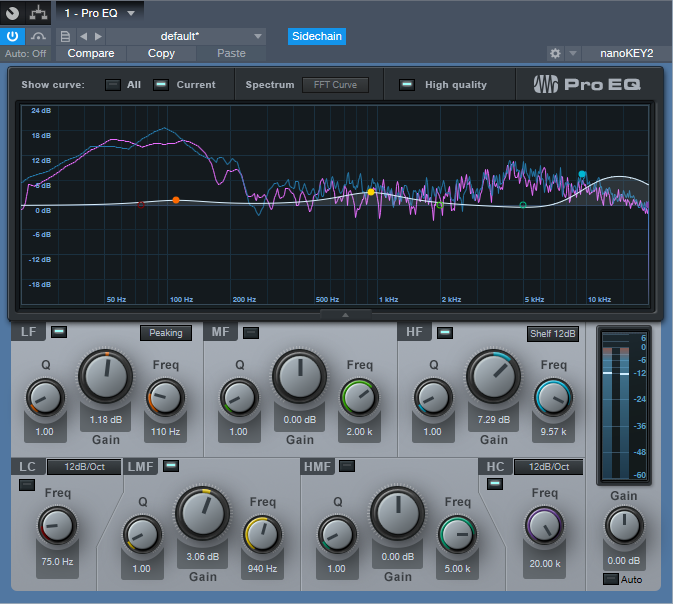
When you enable sidechaining, you can feed another track’s output into the Pro EQ’s spectrum analyzer, while still allowing the Pro EQ to modify the track into which it’s inserted. When sidechained, the Spectrum mode switches to FFT curve (the Third Octave and Waterfall options aren’t available). The blue line indicates the level of the signal going through the Pro EQ, while the violet line represents the sidechain signal.

As a practical example of why this is useful, the screen shot shows two drum loops from different drum loop libraries that are used in the same song. The loop feeding the sidechain loop has the desired tonal qualities, so the loop going through the EQ is being matched as closely as possible to the sidechained loop (as shown by a curve that applies more high end, and a slight midrange bump).

Another example would be when overdubbing a vocal at a later session than the original vocal. The vocalist might be off-axis or further away from the mic, which would cause a slight frequency response change. Again, the Pro EQ’s spectrum meter can help point out any differences by comparing the frequency response of the original vocal to the overdub’s response.

The Spectrum Meter

Sidechaining with the Spectrum Meter provides somewhat different capabilities compared to the Pro EQ’s spectrum analyzer.

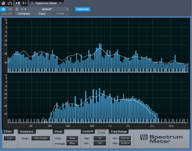
With sidechain enabled, the top view shows the spectrum of the track into which you’ve inserted the Spectrum Meter. The lower view shows the spectrum of the track feeding the sidechain. When sidechained, all the Spectrum Meter analysis modes are available except for Waterfall and Sonogram.

While useful for comparing individual tracks (as with the Pro EQ spectrum meter), another application is to help identify frequency ranges in a mix that sound overly prominent. Insert the Spectrum Meter in the master bus, and you’ll be able to see if a specific frequency range that sounds more prominent actually is more prominent (in the screen shot, the upper spectrum shows a bump around 600 Hz in the master bus). Now you can send individual tracks that may be causing an anomaly into the Spectrum Metre’s sidechain input to determine which one(s) are contributing the most energy in this region. In the lower part of the screen shot, the culprit turned out to be a guitar part with a wah that emphasized a particular frequency. Cutting the guitar EQ just a little bit around 600 Hz helped even out the mix’s overall sound.

Of course, the primary way to do EQ matching is by ear. However, taking advantage of Studio One’s analysis tools can help speed up the process by identifying specific areas that may need work, after which you can then do any needed tweaking based on what you hear. Although “mixing with your eyes” isn’t the best way to mix, supplementing what you hear with what you see can expedite the mixing process, and help you learn to correlate specific frequencies with what you hear—and there’s nothing wrong with that.

One of my favorite techniques for larger-than-life sounds is layering a synthesizer waveform behind a sampled sound. For example, layering a sine wave along with piano or acoustic guitar, then mixing the sine wave subtly in the background, reinforces the fundamental. With either instrument, this can give a powerful low end. Layering a triangle wave with harp imparts more presence to sampled harps, and layering a triangle wave an octave lower with a female choir sounds like you’ve added a bunch of guys singing along.

Another favorite, which we’ll cover in detail with this week’s tip, is layering a sawtooth or pulse wave with strings. I like those syrupy, synthesized string sounds that were so popular back in the 70s, although I don’t like the lack of realism. On the other hand, sampled strings are realistic, but aren’t lush enough for my tastes. Combine the two, though, and you get lush realism. Here’s how.

1. Create an instrument track with Presence, and call up the Violin Full preset.
2. Drag Mai Tai into the same track. You’ll be asked if you want to Replace, Keep, or Combine. Choose Combine.

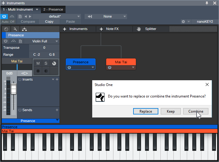
3. After choosing Combine, both instruments will be layered within the Instrument Editor (see above).
4. Program Mai Tai for a very basic sound, because it’s there solely to provide reinforcement—a slight detuning of the oscillators, no filter modulation, very basic LFO settings to add a little vibrato and prevent too static a waveform, amplitude envelope and velocity that tracks the Presence sound as closely as possible, some reverb to create a more “concert hall” sound, etc. The screen shot shows the parameters used for this example. The only semi-fancy programming tricks were making one of the oscillators a pulse wave instead of a sawtooth, and panning the two oscillators very slightly off-center.

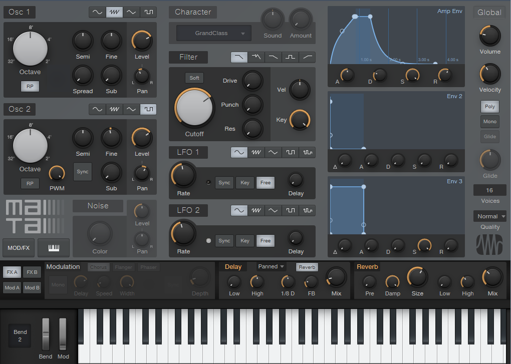
5. Adjust the Mai Tai’s volume for the right mix—enough to supplement Presence, but not overwhelm it.

That’s all there is to it. Listen to the audio example—first you’ll hear only the Presence sound, then the two layers for a lusher, more synthetic vibe that also incorporates some of the realism of sampling. Happy orchestrating!

When Harmonic Editing was announced, I was interested. When I used it for the first time, I was intrigued. When I discovered what it could do for songwriting…I became addicted.

Everyone creates songs differently, but for me, speed is the priority—I record scratch tracks as fast as possible to capture a song’s essence while it’s hot. But if the tracks aren’t any good, they don’t inspire the songwriting process. Sure, they’ll get replaced with final versions later, but you don’t want boring tracks while writing.

For scratch drums on rock projects, I have a good collection of loops. Guitar is my primary instrument, so the rhythm and lead parts will be at least okay. I also drag the rhythm guitar part up to the Chord Track to create the song’s “chord chart.”

Then things slow down…or at least they did before Harmonic Editing came along. Although I double on keyboards, I’m not as proficient as on guitar but also, prefer keyboard bass over electric bass—because I’ve sampled a ton of basses, I can find the sound I want instantly. And that’s where Harmonic Editing comes in.

The following is going to sound ridiculously easy…because it is. Here’s how to put Studio One’s Robot Bassist to work. This assumes you’ve set the key (use the Key button in the transport, or select an Instrument part and choose Event > Detect Key Signature), and have a Chord Track that defines the song’s chord progression.

1. Play the bass part by playing the note on a MIDI keyboard that corresponds to the song’s key. Yes, the note—not notes. For example, if the song is in the key of A, hit an A wherever you want a bass note.
2. Quantize what you played. It’s important to quantize because presumably, the chord changes are quantized, and the note attack needs to fall squarely at the beginning of, or within, the chord change. You can always humanize later.
3. Open the Inspector, unfold the Follow Chords options, and then choose Bass (Fig. 1).

Figure 1: Choose the Bass option to create a bass part when following chords.

4. Now you have a bass part! If the bass part works, choose the Edit tab, select all the notes, and choose Action > Freeze Pitch. This is important, because the underlying endless-string-of-notes remains the actual MIDI data. So if you copy the Event and paste it, unless you then ask the pasted clip to follow chords, you have the original boring part instead of the robotized one.
5. After freezing, turn off Follow Chords, because you’ve already followed the chords. Now is the time to make any edits. (Asking the followed chords to follow chords can confuse matters, and may modify your edits.)

The bottom line: with one take, a few clicks, and (maybe) a couple quick edits—instant bass part (Fig. 2).

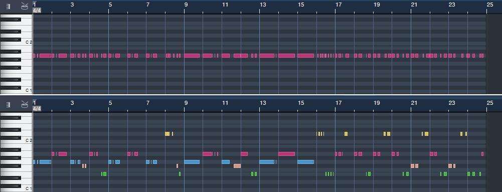
Figure 2: The top image is the original part, and yes, it sounds as bad as it looks. The lower image is what happened after it got robotized via Harmonic Editing, and amazingly, it sounds pretty good.

Don’t believe me? Well, listen to the following.

You’ll hear the bass part shown in Fig. 2, which was generated in the early stages of writing my latest music video (I mixed the bass up a little on the demo so you can hear it easily). Note how the part works equally well for the sustained notes toward the beginning, and well as the staccato parts at the end. To hear the final bass part, click the link for Puzzle of Love [https://youtu.be/HgMF-HBMrks]. You’ll hear I didn’t need to do much to tweak what Harmonic Editing did.

But Wait! There’s More!

Not only that, but most of the backing keyboard parts for Puzzle of Love (yes, including the piano intro) were generated in essentially the same way. That requires a somewhat different skill set than robotizing the bass, and a bit more editing. If you want to know more (use the Comments section), we’ll cover Studio One’s Robot Keyboardist in a future Friday Tip.

Limiters are common mastering tools, so they’re the last processor in a signal chain. Because of this, it’s important to know as much as possible about its output signal, and Studio One’s Limiter offers several metering options.

PkRMS Metering

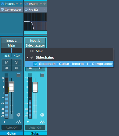
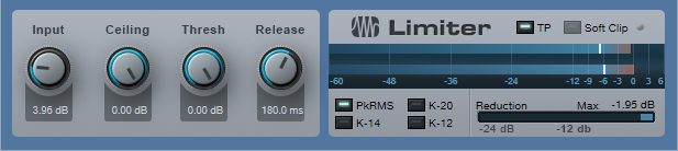
The four buttons under the meter’s lower left choose the type of meter scale. PkRMS, the traditional metering option, shows the peak level as a horizontal blue bar, with the average (RMS) level as a white line superimposed on the blue bar (Fig. 1). The average level corresponds more closely to how we perceive musical loudness, while the bar indicates peaks, which is helpful when we want to avoid clipping.

The TP Button

Enabling the True Peak button takes the possibility of intersample distortion into account. This type of distortion can occur on playback if some peaks use up the maximum available headroom in a digital recording, and then these same peaks pass through the digital-to-analog converter’s output smoothing filter to reconstruct the original waveform. This reconstructed waveform might have a higher amplitude than the peak level of the samples, which means the waveform now exceeds the maximum available headroom (Fig. 2).

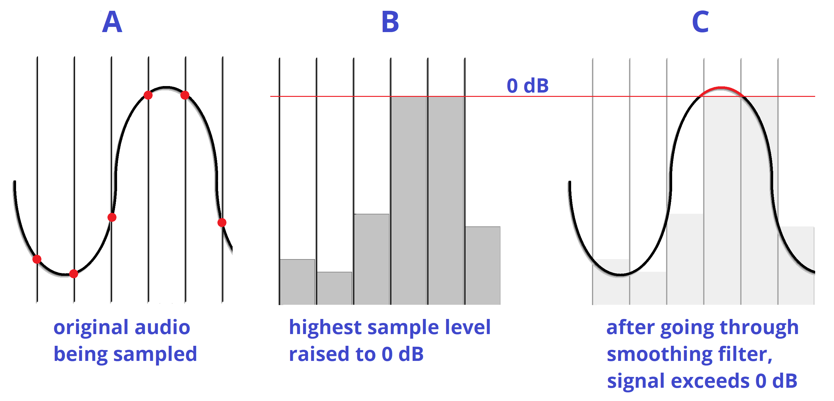
Figure 2: How intersample distortion occurs.

For example, you might think your audio isn’t clipping because without TP enabled, the output peak meter shows -0.1 dB. However, enabling True Peak metering may reveal that the output is as much as +3 dB over 0 when reconstructed. The difference between standard peak metering and true peak metering depends on the program material.

K-System Metering

The other metering options—K-12, K-14, and K-20 metering—are based on a metering system developed by Bob Katz, a well-respected mastering engineer. One of the issues any mix or mastering engineer has to resolve is how loud to make the output level. This has been complicated by the “loudness wars,” where mixes are intended to be as “hot” as possible, with minimal dynamic range. Mastering engineers have started to push back against this not just to retain musical dynamics, but because hot recordings cause listener fatigue. Among other things, the K-System provides a way to judge a mix’s perceived loudness.

A key K-System feature is an emphasis on average (not just peak) levels, because they correlate more closely to how we perceive loudness. A difference compared to conventional meters is that K-System meters use a linear scale, where each dB occupies the same width (Fig. 3). A logarithmic scale increases the width of each dB as the level gets louder, which although it corresponds more closely to human hearing, is a more ambiguous way to show dynamic range.

Figure 3: The K-14 scale has been selected for the Limiter’s output meter.

Some people question whether the K-System, which was introduced two decades ago, is still relevant. This is because there’s now an international standard (based on a recommendation by the International Telecommunications Union) that defines perceived average levels, based on reference levels expressed in LUFS (Loudness Units referenced to digital Full Scale). As an example of a practical application, when listening to a streaming service, you don’t want massive level changes from one song to the next. The streaming service can regulate the level of the music it receives so that all the songs conform to the same level of perceived loudness. Because of this, there’s no real point in creating a hot master—it will just be turned down to bring it in line with songs that retain dynamic range; and the latter will be turned up if needed to give the same perceived volume.

Nonetheless, the K-System remains valid, particularly when mixing. When you mix, it’s best to have a standardized, consistent monitoring level because human hearing has a different frequency response at different levels (Fig. 4).

Figure 4: The Fletcher-Munson curve shows that different parts of the audio spectrum need to be at different levels to be perceived as having the same volume. Low frequencies have to be substantially louder at lower levels to be perceived as having equal volume.

The K-System links monitoring levels with meter readings, so you can be assured that music reaching the same levels will sound like they’re at the same levels. This requires calibrating your monitor levels to the meter readings with a sound level meter. If you don’t have a sound level meter, many smartphones can run sound level meter apps that are accurate enough.

Note that in the K-System, 0 dB does not represent the maximum possible level. Instead, the 0 dB point is shifted “down” from the top of the scale to either -12, -14, or -20 dB, depending on the scale. These numbers represent the amount of headroom above 0, and therefore, the available dynamic range. You choose a scale based on the music you’re mixing or mastering—like -12 for music with less dynamic range (e.g., dance music), -14 for typical pop music, and -20 dB for acoustic ensembles and classical music. You then aim for having the average level hover around the 0 dB point. Peaks that go above this point will take advantage of the available headroom, while quieter passages will go below this point. Like conventional meters, the K-Systems meters have green, yellow, and red color-coding to indicate levels. Levels above 0 dB trigger the red, but this doesn’t mean there’s clipping—observe the peak meter for that.

Calibrating Your Monitors

The K-System borrows film industry best practices. At 0 dB, your monitors should be putting out 85 dBSPL for stereo material. Therefore, you’ll need a separate calibration for the three scales to make sure that 0 dB on any scale has the same perceived loudness. The simplest way to calibrate is to send pink noise through your system until the chosen K-System meter reads 0 dB (you can download pink noise samples from the web, or use the noise generator in the Mai Tai virtual instrument). Then, using the sound level meter set to C weighting and a slow response, adjust the monitor level for an 85 dB reading. You can put labels next to the level control on the back of your speaker to show the settings that produce the desired output for each K-Scale.

But Wait! There’s More

We’ve discussed the K-System in the context of the Limiter, but if you’re instead using the Compressor or some other dynamics processor that doesn’t have K-System metering, you’re still covered. There’s a separate metering plug-in that shows the K-System scale (Fig. 5).

Figure 5: The Level meter plug-in shows K-System as well as the R128 spec that reads out the levels in LUFS. Enabling TP converts the meter to PkRMS, and shows the True Peak in the two numeric fields.

Finally, the Project Page also includes K-System Metering along with a Spectrum Analyzer, Correlation Meter, and LUFS metering with True Peak (Fig. 6).

Figure 6: The Project Page metering tells you pretty much all you need to need to know what’s going on with your output signal when mastering.

If you’ve heard blues harmonica greats like Junior Wells, James Cotton, Jimmy Reed, and Paul Butterfield, you know there’s nothing quite like that big, brash sound. They all manage to transform the harmonica’s reedy timbre into something that seems more like a member of the horn family.

To find out more about the techniques of blues harmonica, check out the article Rediscovering Blues Harmonica. It covers why you don’t play blues harp in its default key (e.g., you typically use a harmonica in the key of A for songs in E), how to mic a harmonica, and more. However, the secret to that big sound is playing through the distortion provided by an amp, or in our software-based world, an amp sim. I don’t really find the Ampire amps suitable for this application, but we can put together an FX Chain that does the job.

Check out the demo to hear the desired goal. The first 12 bars are unprocessed harmonica (other than limiting). The second 12 bars use the FX Chain described in this week’s tip, and which you can download for your own use.

The chain starts with a Limiter to provide a more sustained, consistent sound.

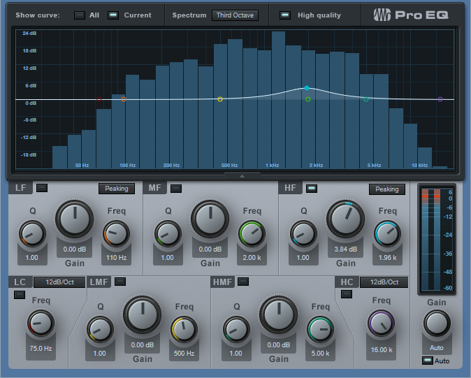
Next up: A Pro EQ to take out all the lows and highs, which tightens up the sound and reduces intermodulation distortion. (When using an amp sim, blues harmonica is also a good candidate for multiband processing, as described in the February 1 Friday Tip.)

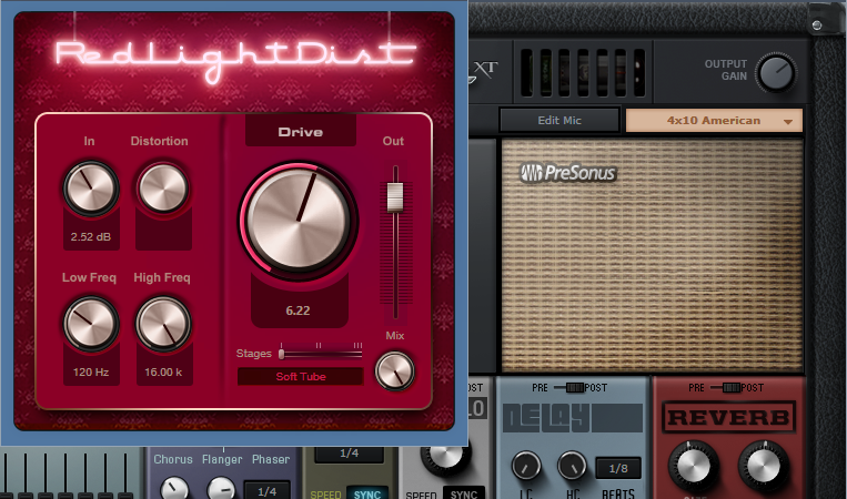
Now it’s time for the Redlight Dist to provide the distortion. For the cabinet, this FX Chain uses the Ampire solely for its 4 x 10 American cabinet—no amp or stomps.

After the distortion/cabinet combo, a little midrange “honk” makes the harmonica stand out more in the mix.

For a final touch, blues harp often plays through an amp with reverb—so a good spring reverb effect adds a vintage vibe.

You can download the Blues Harp.multipreset and use it as it, but I encourage playing around with it—try different types of distortion and amps, mess with the EQ a bit, and so on. For an example of a finished song with amp sim blues harmonica in context, check out I’ll Take You Higher on YouTube.

Click here to download the multipreset!

Although vinyl represents a tiny fraction of the media people use to listen to music, you, or a client, may want to do a vinyl release someday. Conventional wisdom is split between “you don’t dare master for vinyl” and “sure, you can master for vinyl if you know certain rules.”

Both miss the point that the engineer using the lathe to do the cutting will make the ultimate decisions. You can provide something mastered for CD, and the engineer will do what’s possible to make it vinyl-friendly—but then the vinyl version may sound very different from the CD, because of the compromises needed to accommodate vinyl. Conversely, you can “prep for vinyl” and if you do a good job, the engineer running the cutting lathe will have an easier time, and there won’t be as much difference between the vinyl and CD release.

But before going any further, let’s explore why vinyl is different.

TRADEOFFS

A stylus moves side to side, and up and down, to create stereo. Louder levels mean wide and deeper grooves; if too loud, the needle can jump out of the groove. Lower frequencies hog “groove space” more than high frequencies, but also, a stylus has a difficult time moving fast enough to track high frequencies, which leads to distortion.

To compensate, the RIAA initiated an EQ curve that cuts bass up to -20 dB at low frequencies before the audio gets turned into a master lacquer, and boosts highs by an equally dramatic amount to help overcome surface noise. On playback, an inverse curve boosts the bass to restore its original level; cutting highs restores the proper high-frequency balance to reduce surface noise and encourage better tracking (Fig. 1).

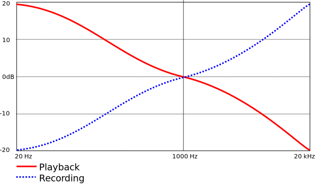
Figure 1: RIAA equalization record and playback curves for vinyl records.

PREPARATION IN THE SONG PAGE

There are four main ways to make more vinyl-friendly mixes in the Song Page.

1. Avoid excessive high frequencies. Use de-essing on vocals, but de-essing can also tame distorted guitar, cymbals, and other high-frequency sound sources (Fig. 2). Excess sibilance or brightness translates to splattering distortion with vinyl.

Figure 2: Studio One’s compressor can do de-essing and other frequency-selective compression.

2. Trim the lows and highs, as appropriate for the program material. Use a 48 dB/octave Pro EQ LC filter to cut everything below 20 to 40 Hz. Back in the vinyl days, sharp cuts above 15 kHz or even 10 kHz were also the norm (Fig. 3).

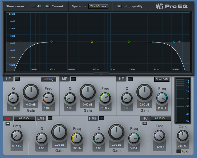
Figure 3: Sharp LC and HC filters trim out vinyl-hostile frequencies.

3. Center the bass. The worst-case audio for a stylus to track is out-of-phase bass in the left and right channels. Besides, low frequencies aren’t very directional, so any stereo is more or less pointless unless you’re listening on headphones. The easiest way to center bass in Studio One is to place a Splitter in the master bus, and split by frequency. There is no “rule” for the correct crossover frequency; too low, and potentially problematic frequencies can get through. Too high, and you’ll start interfering with the lower end of guitar and other instruments. That said, 70 to 170 Hz is a good place to start. Then, follow that low split with the Dual Pan, and center both channels (Fig. 4). Also consider avoiding hard left/right panning for lower-frequency instruments, like toms.

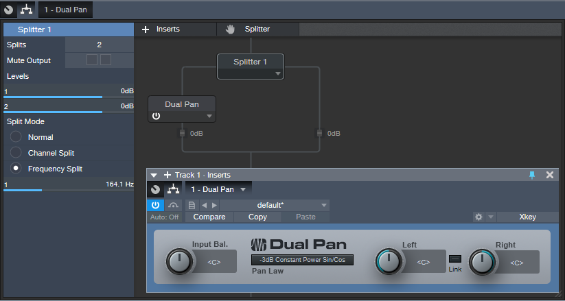
Figure 4: Using a Splitter as a crossover, with a Dual Pan, can center low frequencies in the stereo spread.

4. Check your mix in mono. Phase issues, whether accidental or deliberate (i.e., psycho-acoustic processors) can really mess with the cutting lathe. Use Studio One’s Correlation meter to confirm there aren’t major phase issues (see the Friday Tip for September 28, 2018).

PREPARATION IN THE PROJECT PAGE

You can take matters only so far in the Project Page before taking your mixes to a mastering engineer who knows how to prep for, and cut, vinyl. But there are steps you should take to assist the process of creating a vinyl-friendly master for duplication.

1. Follow the rules for album length. The two sides should be of approximately equal length, and for a 12” record, should not exceed 20 minutes. Longer sides mean narrower grooves, lower levels, and more issues with surface noise. There’s a reason why many classic albums were 30-40 minutes long total.
2. Follow the rules for album order. Fidelity deteriorates as the stylus works its way toward the inner grooves. Place your loudest songs, with the most complex spectra, at the beginning of a side, and the quieter songs toward the end. This may require choosing whether you want to compromise your art, or the sound quality.
3. Don’t try to win the loudness wars. You can ask the engineer cutting the vinyl to put as loud a level as possible on vinyl, but don’t try it yourself. Loud, distorted or partially clipped audio only sounds worse when translated to vinyl because the stylus can’t follow clipped waveforms easily. Think about it—a mechanical object can’t snap to a maximum value and then back down to a lower value instantly. What matters is the average, not peak, level; I master to around -10 or -11 LUFS these days, and that works for vinyl. You can maybe stretch that to -8 with some material, but the louder you go, the greater the chance of distortion.
4. Create a complete, continuous disc image file (Fig. 5) that represents exactly what you want each side to sound like. The process of transferring from a final mix to a cutting lathe is done in real time. The image should include the desired silence between cuts, crossfades, and song order. Of course you can have a mastering engineer assemble the album from individual cuts, but you’ll pay extra.

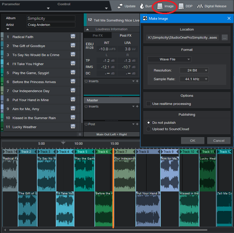
Figure 5: I mastered my 2017 album project, Simplicity, with vinyl in mind “just in case.” The total length is about 31 minutes, and the project splits into two sides of almost equal length between songs 6 and 7 (shown with an orange line). An image of the entire project is about to be created.

5. Get a reference lacquer. You’ll pay extra for this, but it lets you “proof” the settings the mastering engineer uses to create the final master lacquer. You can play the reference at least a dozen or more times before the quality starts to deteriorate audibly. If changes need to be made, the mastering engineer will have written down the settings used to make the reference, and re-adjust them as needed.

SO THAT’S WHY VINYL SOUNDS BETTER!!

Yes. Properly mastered vinyl releases didn’t have harsh high frequencies, they had dynamic range because you couldn’t limit the crap out of them without having them sound distorted, and the bass coalesced around the stereo image’s center, where it belongs. In fact, if you master with vinyl in mind, you just might find that those masters make CDs sound a whole lot better as well!

I’m a big fan of multiband processing. This technique divides a signal into bands (I generally choose lows, low mids, mids, and high mids), processes each band independently, then sums the bands’ outputs back together again.

I first used multiband processing in the early 80s, with the Quadrafuzz distortion unit (later virtualized by both Steinberg and MOTU). This produces a “cleaner” distortion sound because you didn’t have the intermodulation distortion caused by low strings and high strings interacting with each other. However, multiband processing is also useful with delay, like using shorter delays on lower frequencies, and longer delays on higher frequencies…or chorus, if you want a super-lush sound. But there are other cool surprises, like using different effects in the different bands, or using envelope filters.

So for Studio One, I’ve created a multiband processing “development system” for creating new multiband effects—and that’s the subject of this tip.When I find an effect I like, it gets turned into a fixed FX chain that uses the Splitter module’s multi-band capabilities instead of buses to create four parallel signal paths.

Band Splitting

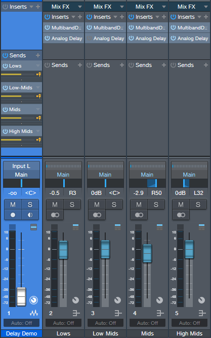
Figure 1: The Multiband Processing Development System, set to evaluate multiband processing with analog delay.

Start by creating four pre-fader sends to feed four buses (fig. 1). Each bus handles a specific frequency range. The simplest way to create splits is with the Multiband Dynamics set to no compression, so it can serve as a crossover.

To create the bands, insert a Multiband Dynamics processor in one of the buses, open it, and set the compression Ratio for all Multiband Dynamics bands to 1:1. This prevents any compression from occurring.

Referring to fig. 2, as you play your instrument (or other signal source you want to process), solo the Low band. Then adjust the Low / Low-Mid X-Over Frequency control to set the dividing frequency between the low- and low-mid band.

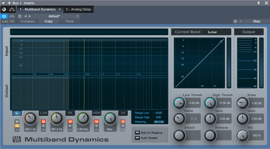
Figure 2: Use the Multiband Dynamics processor to create the individual band in each bus.

Next, solo the Low Mid band and adjust its frequency control. Use a similar procedure on each band until you’ve chosen the frequencies you want each band to cover. For guitar, having more than four bands isn’t all that necessary, so I normally set the frequency splits to around 250 Hz, 500 Hz, and 1 kHz. The resulting bands are:

• Below 250 Hz
• 250 – 500 Hz
• 500 – 1,000 Hz
• Above 1,000 Hz

Setting the Mid-High / High X-Over Frequency to Max essentially removes the Multiband Dynamics’  top band.

After choosing the frequency bands, copy the Multiband Dynamics processor to the other three buses. Solo the Low band for one bus, the Low Mid in the next bus, the Mid in the next bus, and finally, the High Mids in the fourth bus. Now each bus covers its assigned frequency range.

At this point, all that’s left is to insert your processor(s) of choice into each band. Don’t forget that you can experiment with panning the different bands, changing levels, altering sends to the buses to affect distortion drive, and more. This type of setup allows for a ton of options…so get creative!

I was never a big fan of MIDI guitar, but that changed when I discovered two guitar-like controllers—the YRG1000 You Rock Guitar and Zivix Jamstik. Admittedly, the YRG1000 looks like it escaped from Guitar Hero to seek a better life, but even my guitar-playing “tubes and Telecasters forever!” compatriots are shocked by how well it works. And Jamstik, although it started as a learn-to-play guitar product for the Mac, can also serve as a MIDI guitar controller. Either one has more consistent tracking than MIDI guitar retrofits, and no detectable latency.

The tradeoff is that they’re not actual guitars, which is why they track well. So, think of them as alternate controllers that take advantage of your guitar-playing muscle memory. If you want a true guitar feel, with attributes like actual string-bending, there are MIDI retrofits like Fishman’s clever TriplePlay, and Roland’s GR-55 guitar synthesizer.

In any case, you’ll want to set up your MIDI guitar for best results in Studio One—here’s how.

Poly vs. Mono Mode

MIDI guitars usually offer Poly or Mono mode operation. With Poly mode, all data played on all strings appears over one MIDI channel. With Mono mode, each string generates data over its own channel—typically channel 1 for the high E, channel 2 for B, channel 3 for G, and so on. Mono mode’s main advantage is you can bend notes on individual strings and not bend other strings. The main advantage of Poly mode is you need only one sound generator instead of a multi-timbral instrument, or a stack of six synths.

In terms of playing, Poly mode works fine for pads and rhythm guitar, while Mono mode is best for solos, or when you want different strings to trigger different sounds (e.g., the bottom two strings trigger bass synths, and the upper four a synth pad). Here’s how to set up for both options in Studio One.

1. To add your MIDI guitar controller, choose Studio One > Options > External Devices tab, and then click Add…
   

   Figure 1: Check “Split Channels” if you plan to use a MIDI guitar in mono mode.

   2. To use your guitar in Mono mode, check Split Channels and make sure All MIDI channels are selected (Fig. 1). This lets you choose individual MIDI channels as Instrument track inputs.

    

   3. For Poly mode, you can follow the same procedure as Mono mode but then you may need to select the desired MIDI channel for an Instrument track (although usually the default works anyway). If you’re sure you’re going to be using only Poly mode, don’t check Split Channels, and choose the MIDI channel over which the instrument transmits.

   Note that you can change these settings any time in the Options > External Devices dialog box by selecting your controller and choosing Edit.

   Choose Your Channels

   For Poly mode, you probably won’t have to do anything—just start playing. With Mono mode, you’ll need to use a multitimbral synth like SampleTank or Kontakt, or six individual synths. For example, suppose you want to use Mai Tai. Create a Mai Tai Instrument track, choose your MIDI controller, and then choose one of the six MIDI channels (Fig. 2). If Split Channels wasn’t selected, you won’t see an option to choose the MIDI channel.

   

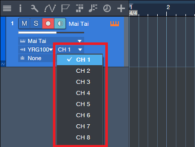
   Figure 2: If you chose Split Channels when you added your controller, you’ll be able to assign your instrument’s MIDI input to a particular MIDI channel.

   Next, after choosing the desired Mai Tai sound, duplicate the Instrument track five more times, and choose the correct MIDI channel for each string. I like to Group the tracks because this simplifies removing layers, turning off record enable, and quantizing. Now record-enable all tracks, and start recording. Fig. 3 shows a recorded Mono guitar part—note how each string’s notes are in their own channel.

   

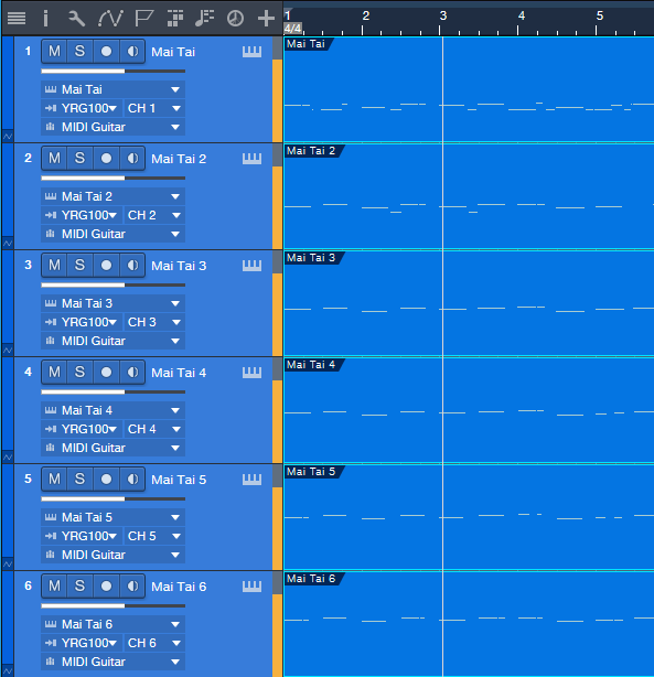
   Figure 3: A MIDI guitar part that was recorded in Mono mode is playing back each string’s notes through its own Mai Tai synthesizer.

   To close out, here are three more MIDI guitar tips.

   • In Mono mode with Mai Tai (or whatever synth you use), set the number of Voices to 1 for two reasons. First, this is how a real guitar works—you can play only one note at a time on a string. Second, this will often improve tracking in MIDI guitars that are picky about your picking.
   • Use a synth’s Legato mode, if available. This will prevent re-triggering on each note when sliding up and down the neck, or doing hammer-ons.
   • The Edit view is wonderful for Mono mode because you can see what all six strings are playing, while editing only one.

   MIDI guitar got a bad rap when it first came out, and not without reason. But the technology continues to improve, dedicated controllers overcome some of the limitations of retrofitting a standard guitar, and if you set up Studio One properly, MIDI guitar can open up voicings that are difficult to obtain with keyboards.

   In Mono mode with Mai Tai (or whatever synth you use), set the number of Voices to 1 for two reasons. First, this is how a real guitar works—you can play only one note at a time on a string. Second, this will often improve tracking in MIDI guitars that are picky about your picking.