I sometimes record acoustic rhythm guitars with one mic for two main reasons: no issues with phase cancellations among multiple mics, and faster setup time. Besides, rhythm guitar parts often sit in the background, so some ambiance with electronic delay and reverb can give a somewhat bigger sound. However, on an album project with the late classical guitarist Linda Cohen, the solo guitar needed to be upfront, and the lack of a stereo image due to using a single mic was problematic.

Rather than experiment with multiple mics and deal with phase issues, I decided to go for the most accurate sound possible from one high-quality, condenser mic. This was successful, in the sense that moving from the control room to the studio sounded virtually identical; but the sound lacked realism. Thinking about what you hear when sitting close to a classical guitar provided clues on how to obtain the desired sound.

If you’re facing a guitarist, your right ear picks up on some of the finger squeaks and string noise from the guitarist’s fretting hand. Meanwhile, your left ear picks up some of the body’s “bass boom.” Although not as directional as the high-frequency finger noise, it still shifts the lower part of the frequency spectrum somewhat to the left. Meanwhile, the main guitar sound fills the room, providing the acoustic equivalent of a center channel.

Sending the guitar track into two additional buses solved the imaging problem by giving one bus a drastic treble cut and panning it somewhat left. The other bus had a drastic bass cut and was panned toward the right (Fig. 1).

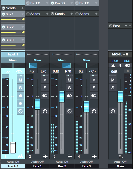
Figure 1: The main track (toward the left) splits into three pre-fader buses, each with its own EQ.

One send goes to bus 1. The EQ is set to around 400 Hz (but also try lower frequencies), with a 24 dB/octave slope to focus on the guitar body’s “boom.” Another send goes to bus 2, which emphasizes finger noises and high frequencies. Its EQ has a highpass filter response with a 24dB/octave slope and frequency around 1 kHz. Pan bus 1 toward the left and bus 2 toward the right, because if you’re facing a guitarist the body boom will be toward the listener’s left, and the finger and neck noises will be toward the listener’s right.

The send to bus 3 goes to the main guitar sound bus. Offset its highpass and lowpass filters a little more than an octave from the other two buses, e.g., 160 Hz for the highpass and 2.4 kHz for the lowpass (Fig. 2). This isn’t “technically correct,” but I felt it gave the best sound.

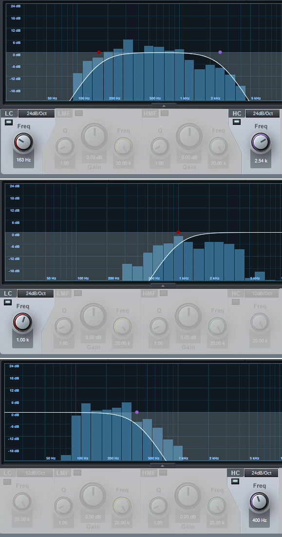
Figure 2: The top curve trims the response of the main guitar sound, the middle curve isolates the high frequencies, and the lower curve isolates the low frequencies. EQ controls that aren’t relevant are grayed out.

Monitor the first two buses, and set a good balance of the low and high frequencies. Then bring up the third send’s level, with its pan centered. The result should be a big guitar sound with a stereo image, but we’re not done quite yet.

The balance of the three tracks is crucial to obtaining the most realistic sound, as are the EQ frequencies. Experiment with the EQ settings, and consider reducing the frequency range of the bus with the main guitar sound. If the image is too wide, pan the low and high-frequency buses more to center. It helps to monitor the output in mono as well as stereo for a reality check.

Once you nail the right settings, you may be taken aback to hear the sound of a stereo acoustic guitar with no phase issues. The sound is stronger, more consistent, and the stereo image is rock-solid.

Mid-side (M-S) processing encodes a standard stereo track into a different type of stereo track with two separate components: the left channel contains the center of the stereo spread, or mid component, while the right channel contains the sides of the stereo spread—the difference between the original stereo file’s right and left channels (i.e., what the two channels don’t have in common). You can then process these components separately, and after processing, decode the separated components back into conventional stereo.

Is that cool, or what? It lets you get “inside the file,” sometimes to where you can almost remix a mixed stereo file. Need more kick and bass? Add some low end to the center, and it will leave the rest of the audio alone. Or bring up the level of only the sides to make the stereo image wider.

The key to M-S processing is the Mixtool plug-in, and its MS Transform button. The easiest way to get started with M-S processing is with the MS-Transform FX Chain (Fig. 1), found in the Browser’s FX Chains Mixing folder.

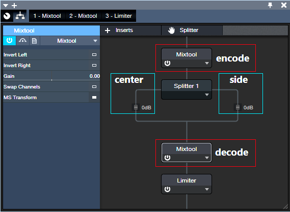
Figure 1: The MS-Transform FX Chain included with Studio One.

The upper Mixtool encodes the signal so that the left channel contains a stereo file’s center component, while the right channel contains the stereo file’s side components. This stereo signal goes to the Splitter, which separates the channels into the side and center paths. These then feed into the lower Mixtool, which decodes the M-S signal back into stereo. (The Limiter isn’t an essential part of this process, but is added for convenience.)

Even this simple implementation is useful. Turn up the post-Splitter gain slider in the Center path to boost the bass, kick, vocals, and other center components. Or, turn up the gain slider in the post-SplitterSide path to bring up the sides, for the wider stereo image we mentioned.

Fig. 2 shows a somewhat more developed FX Chain, where a Pro EQ boosts the highs on the sides. Boosting the highs adds a sense of air, which enhances the stereo image because highs are more directional.

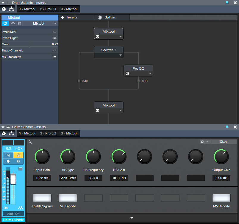
Figure 2: The Image Enhancer FX Chain.

In addition to decoding the signal back to stereo, the second Mixtool has its Output Gain control accessible to compensate for any level differences when the FX Chain is bypass/enabled. Also, you can disable the MS Decoder (last button, lower right) to prevent converting the signal back into stereo, which makes it easy to hear what’s happening in the center and sides.

And of course…you can take this concept much further. Add a second EQ in the center channel, or a compressor if you want to squash the kick/snare/vocals a bit while leaving the sides alone. Try adding reverb to the sides but not the center, to avoid muddying what’s happening in the center. Or, add some short delays to the sides to give more of a room sound….the mind boggles at the possibilities, eh?

Download the Image Enhancer FX Chain here! 

Spoiler alert: We’ll get into some rocket science stuff here, which probably doesn’t affect your projects much anyway…so if you prefer something with a more musical vibe, come back next week. But to dispel some of the confusion regarding an oft-misunderstood concept, keep reading.

You pan a mono signal from left to right. Simple, right? Actually, no. In the center, there’s a 3 dB RMS volume buildup because the same signal is in both channels. Ideally, you want the signal’s average level—its power—to have the same perceived volume, whether the sound is panned left, right, or center. Dropping the level when centered by 3 dB RMS accomplishes this. As a result, traditional hardware mixers tapered the response as you turned a panpot to create this 3 dB dip.

However, there are other panning protocols. (Before your head explodes, please note you don’t need to learn all this stuff—it’s just to give you an idea of the complexity of pan laws, because all we really need to do is understand how things work in Studio One.) For example, some engineers preferred more of a drop in the center, so that audio panned to the sides would “pop” more due to the higher level, and open up more space in the center for vocals, kick, and bass. You could accomplish the same result by adjusting the channel level and pan, but the additional drop was sort of like having a preference you didn’t need to think about. To complicate matters further, some mixers lowered the center signal compared to the sides, while others raised the side signals compared to the center. If a DAW does the latter, when you import a normalized file and pan it hard left or hard right, it will go above 0 and clip.

But wait! There’s more. Some engineers didn’t want equal power over the panpot’s entire travel, but a slightly different curve. Others wanted a linear change that didn’t dip the signal at all.

Fortunately, Studio One has a rational approach to pan laws, namely…

• The panpots in Studio Once’s channels default to the traditional 3 dB dip, so there’s perceived constant level as you pan a mono signal from left to right. For stereo, they act as a balance control.
• Although most programs set the pan law as a global preference, Studio One includes the Dual Pan plug-in, which offers five different pan laws. This lets different channels follow different pan laws.

THE “WHAT-THE-HECK-DO-PAN-LAWS-DO” TEST SETUP

To see how the different panning laws affect signal levels, I created a test setup (Fig. 1) with a mono track fed by the Tone Generator set to a sine wave. Two pre-fader sends went to two buses, each with a Dual Pan inserted and linked for mono. That way, one bus’s Dual Pan could be set for hard pan and the other bus’s Dual Pan for center, to compare what happens to the signal level.

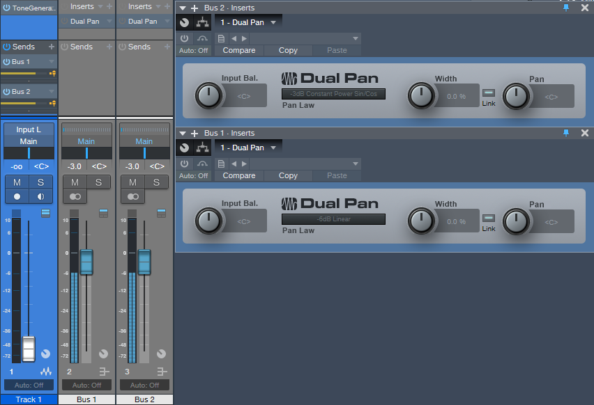
Figure 1: Test setup to determine how different pan laws affect signal levels.

In all the following test result images, Track 1 shows the mono sine wave at 0 dB, Bus 1 shows the result of panning the Dual Pan full left, and Bus 2 shows the result of panning the Dual Pan to center.

Fig. 2 uses the -3dB Constant Power Sin/Cos setting for the Dual Pans. Note that the centered version in Bus 2 is 3 dB below the same signal panned full left. This is the same setting as the default for the channel panpots. However, if you collapse the output signal to mono, you’ll get a 3 dB center-channel buildup. (A fine point: setting the Main bus mode to mono affects signals leaving the main bus; the meters still show the incoming signal. To see what’s happening when you collapse the Main out to mono, you need to insert a Dual Pan in the Main bus, click on Link, and set all controls to center.)

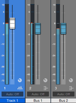
Figure 2: -3dB Constant Power Sin/Cos pan law.

Fig. 3 uses the -6 dB linear curve. Here, the centered signal is -6 dB below the signal panned hard left. Use this curve if the signal is going to be collapsed to mono after the main bus, because it keeps the gain constant when you collapse stereo to mono by eliminating the +3 dB increase that would happen otherwise.

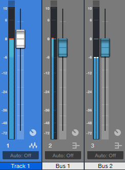
Figure 3: The -6 dB linear curve is often preferable if you’re mixing in stereo, but also anticipate that the final result will end up being collapsed to mono.

Fig. 4 shows the resulting signal from the 0dB Balanced Sin/Cos setting. There’s no bump or decrease compared to the centered signal, so this acts like a balance control with a constant amount of gain as you pan from left to right.

Figure 4:  0dB Balanced Sin/Cos acts like a balance control.

Sharp-eyed readers who haven’t dozed off yet may have noticed we haven’t covered two variations on the curves described so far. -3dB Constant Power Sqrt (Fig. 5; Sqrt stands for Square Root) is like the ‑3 dB Constant Power Sin/Cos, but the curve is subtly different.

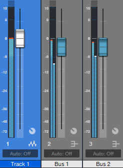
Figure 5: -3dB Constant Power Sqrt bends the curve shape slightly compared to the other Constant Power curve.

In this example, the panpot is set to 75% left instead of full left. Bus 1 shows what happens with -3dB Constant Power Sin/Cos, while Bus 2 is the Sqrt version. The Sqrt version is in less of a hurry to attenuate the right channel as you pan toward the left. Some engineers feel this more closely the situation in a space that’s not acoustically treated, so there’s a natural acoustic center buildup.

Finally, Fig. 6 compares the 0 dB Balance variations, sin/cos and linear.

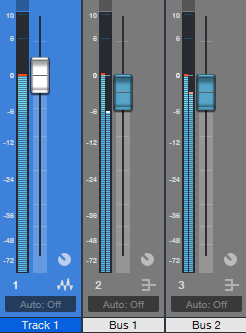
Figure 6: Comparing the two 0 dB Balance pan law options.

The difference is similar to the Constant Power examples, in that the basic idea is the same, but again, the linear version doesn’t attenuate the right channel as rapidly when you pan left.

I HAVEN’T FALLEN ASLEEP YET, SO PLEASE, JUST TELL ME WHAT I SHOULD USE!

The bottom line is when using the channel panpot with a mono track, if you live in a stereo mixdown world the above is mostly of academic interest. But if you’re mixing in stereo and know that your mix will be collapsed to mono (e.g., for broadcast), consider using the Dual Pan in mono channels, and set it to the -6 dB Linear pan law.

For stereo audio, again, a channel panpot works as it should—it acts like a balance control. However if the output is going to be collapsed into mono, you might want to leave the channel panpot centered, and insert a Dual Pan control to do the panning. It should be set to -6 dB Linear, controls unlinked, and then you move both controls equally to pan (e.g., if you want the sound slightly right of center, set both the left and right panpots to 66% right). Now when you pan, the mono levels in the main bus will be constant.

ONE MORE TAKEAWAY…

And finally…I’m sure you’ve seen people on the net who swear that DAW “A” sounds better than DAW “B” because they exported the tracks from one DAW, brought them into a second DAW, set the channel faders and panpots the same, and then were shocked that the two DAWs didn’t sound identical. And for further proof, they note that after mixing down the outputs and doing a null test, the outputs didn’t null. Well, maybe that proves that DAWs are different…but maybe what it really proves is that different programs default to different pan laws, so of course, there are bound to be differences in the mixes.

Well…maybe it actually is, and we’ll cover both positive and negative flanging (there’s a link to download multipresets for both options). Both do true, through-zero flanging, which sounds like the vintage, tape-based flanging sound from the late 60s.

The basis of this is—surprise!—our old friend the Autofilter (see the Friday Tip for June 17, Studio One’s Secret Equalizer, for information on using its unusual filter responses for sound design). The more I use that sucker, the more uses I find for it. I’m hoping there’s a dishwashing module in there somewhere…meanwhile, for this tip we’ll use the Comb filter.

Positive Flanging

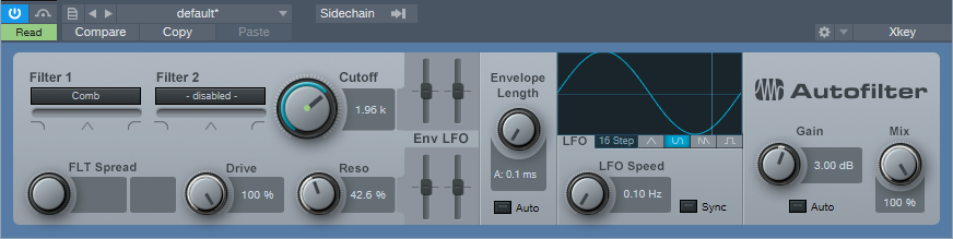
Figure 1: When set properly, the Autofilter’s comb filter can make a superb flanger.

Flanging depended on two signals playing against each other, with the time delay of one varying while the other stayed constant. Positive flanging was the result of the two signals being in phase. This gave a zinging, resonant type of flanging sound.

Fig. 1 shows the control settings for positive flanging. Turn Auto Gain off, Mix to 100%, and set both pairs of Env and LFO sliders to 0. Adding Drive gives a little saturation for more of a vintage tape sound (or follow the May 31 tip, In Praise of Saturation, for an alternate tape sound option). Resonance is to taste, but the setting shown above is a good place to start. The Gain control setting of 3 dB isn’t essential, but compensates for a volume loss when enabling/bypassing the FX Chain.

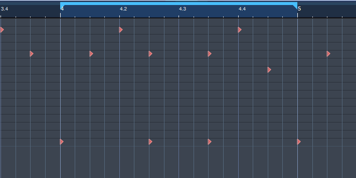
Varying the Cutoff controls the flanging effect. We won’t use the Autofilter’s LFO, because real tape flanging didn’t use an LFO—you controlled it by hand. Controlling the flanging process was always inexact due to tape recorder motor inertia, so a better strategy is to automate the Cutoff parameter, and create an automation curve that approximates the way flanging really varied (Fig. 2)—which was most definitely not a sine or triangle wave. A major advantage of creating an automation curve is that we can make sure that the flanging follows the music in the most fitting way.

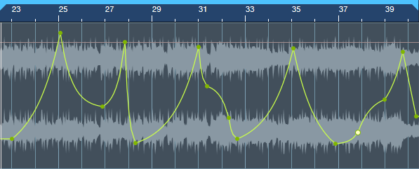
Figure 2: The Cutoff frequency automation curve used for the audio examples.

Negative Flanging

Throwing one of the two signals used to create flanging out of phase gave negative flanging, which had a hollower, “sucking” kind of sound. Also, when the variable speed tape caught up with and matched the reference tape, the signal canceled briefly due to being out of phase. It’s a little more difficult to create negative flanging, but here’s how to do it.

1. Set up flanging as shown in the previous example, and then Duplicate Track (Complete), including the Autofilter.
2. Turn Resonance all the way down in both Autofilters (original and duplicated track). This is important to obtain the maximum negative flanging effect. Because of the cancellation due to the two audio paths being out of phase, there’s a level drop when flanging. You can compensate by turning up both Autofilters’ Gain controls to exactly 6.00 dB (they need to be identical). This gain increase isn’t strictly necessary, but helps maintain levels between the enabled and bypassed states of the Negative Flanging FX Chain.
3. In the duplicated track’s Autofilter, turn off the Autofilter’s Automation Read, and turn Cutoff up all the way (Fig. 3).

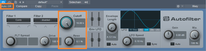
Figure 3: Settings for the duplicated track’s Autofilter.

4. Insert a Mixtool after the Autofilter in the duplicated track, and enable both Invert Left and Invert Right (Fig. 4). This throws the duplicated track out of phase.

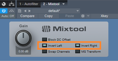
Figure 4: Mixtool settings for the duplicated track.

5. Temporarily bypass both Autofilters (in the original and duplicated tracks). Start playback, and you should hear nothing because the two tracks cancel. If you want to make sure, vary one of the track faders to see if you hear anything, then restore the fader to its previous position.
6. Re-enable both Autofilters, and program your Cutoff automation for the original track (the duplicated track shouldn’t have automation). Note that if you mute the duplicate track, or bring down its fader, the sound will be positive flanging (although with less level than negative flanging, because you don’t have two tracks playing at once).

So is this the best flanger plug-in ever? Well if not, it’s pretty close…listen to the audio examples, and see what you think.

Both examples are adapted/excerpted from the song All Over Again (Every Day).

The Multipresets

If you like what you hear, download the multipresets. There are individual ones for Positive Flanging and Negative Flanging. To automate the Flange Freq knob, right-click on it and choose Edit Knob 1 Automation. This overlays an automation envelope on the track that you can edit as desired to control the flanging.

Download the Positive Flanging Multipresets Here! 

Download the Negative Flanging Multipresets Here! 

And here’s a fine point for the rocket scientists in the crowd. Although most flangers do flanging by delaying one signal compared to another, most delays can’t go all the way up to 0 ms of delay, which is crucial for through-zero flanging where the two signals cancel at the negative flanging’s peak. The usual workaround is to delay the dry signal somewhat, for example by 1 ms, so if the minimum delay time for the processed signal is 1 ms, the two will be identical and cancel. The advantage of using the comb filter approach is that there’s no need to add any delay to the dry signal, yet they can still cancel at the peak of the flanging.

Finally, I’d like to mention my latest eBook—More Than Compressors – The Complete Guide to Dynamics in Studio One. It’s the follow-up to the book How to Record and Mix Great Vocals in Studio One. The new book is 146 pages, covers all aspects of dynamics (not just the signal processors), and is available as a download for $9.99.

Shakers, tambourines, eggs, maracas, and the like can add life and interest to a song by complementing the drum track. But it’s not always easy to play this kind of part. It has to be consistent, but not busy; humble enough to stay in the background, but strong enough to add impact…and this sounds like a job for version 4.5’s new MIDI features.

We’ll go through the process of creating a cool, 16th-note-based percussion part, but bear in mind that this is just one approach. Although it works well, there are many ways you can modify this process (which we’ll touch on at the end).

First, Choose Your Sound

Ideally, you’ll have a couple different samples of the percussion instrument you want to use. But if you don’t, there’s a simple workaround. I use Impact for these kinds of parts, and if there’s only one sample of something like a shaker, I’ll drag it to two pads, and detune one of the pads by -1 semitone so they sound different. In the following example, we’ll call the original sample Sound 1, and detuned sample, Sound 2.

The Process

Let’s create a two-bar percussion loop to start. Grab the Draw tool, and set the Quantize value to 1/4. Drag across the two measures to create a hit at every quarter note for Sound 1 (Fig. 1).

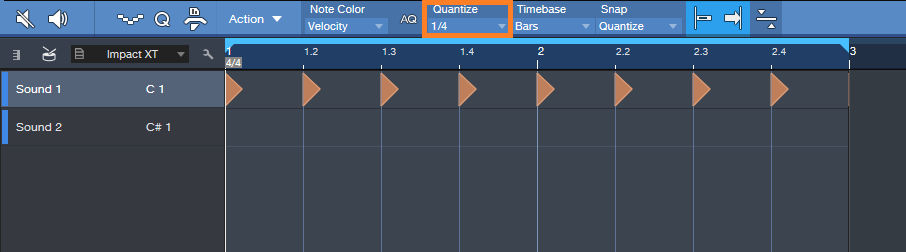
Figure 1. Having a constant series of 1/4-note hits anchors the rhythm so we can alter other hits.

Next, set the Quantize value to 1/16. Drag across the two measures to create a hit at every 16th note for Sound 2 (Fig. 2). Hit Play, so you can marvel at how totally unmusical it sounds.

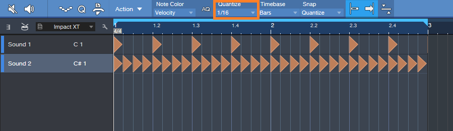
Figure 2: We’ll be modifying the series of 16th notes to add interest.

Now let’s make the part sound good. The key here is not to alter the 1/4 note hits—we want them rock solid, so that the rhythm won’t get pulled too far astray when we start adding variations to the 16th notes.

Select only the 16th notes for Sound 2, and let’s use version 4.5’s new Thin Out Notes command. I’m a fan of Delete notes randomly, and we’ll delete 40% of the notes. Choose the 1/16 grid, since that matches the part. Click OK, and now the part isn’t quite so annoyingly constant (Fig. 3).

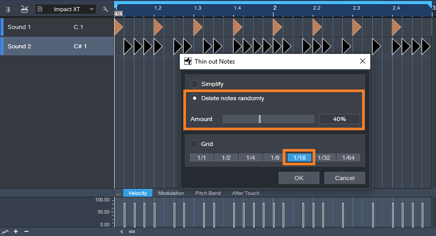
Figure 3: Dropping out the occasional random note adds interest.

But we still need to do something about the velocity, which is way too consistent—the real world doesn’t work that way. Select the string of 16th notes again, and this time, choose Humanize. Set a Velocity range and Note start range (like -40/40% and -.0015/0.0015 respectively), and then click OK (Fig. 4). Now look at the velocity strip: it’s a lot more interesting. The timing changes are also helpful, but they don’t have the “drunken percussion player” quality that you get a lot with randomized timings, because those rock-solid quarter note hits are still establishing the beat.

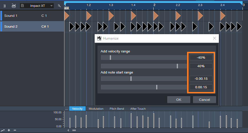
Figure 4: Humanizing velocity and start times for only the 16th notes adds variations that make the part more lively.

So now we have an interesting two-measure loop, but let’s not loop it—instead, we’ll create a part that lasts as long as we want, and it will still be interesting. Here’s how.

Duplicate the two measures for as long as you want. Select all the notes in the Sound B row, and choose Randomize notes. Uncheck everything except Shuffle Notes. Click on OK. All the notes will stay in the same position, and because there are no other candidate notes for shuffling, the timing won’t change. What will Shuffle is velocity. If you created a Shuffle Macro for the May 24 tip on End Boring MIDI Drum Parts, it will come in handy here—keep hitting that macro until the pattern is the way you want. After you de-select the notes, if you’ve chosen Velocity for note color, you’ll have a pretty colorful velocity strip (Fig. 5).

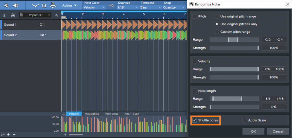
Figure 5: Shuffling velocity in a longer part adds more interesting dynamics.

Now you have a part that sounds pretty good, and once you become familiar with the process, you’ll find it takes less time to generate a part than it does to read this. Here are some options to this technique.

• Instead of creating a short loop, duplicating it, and then shuffling velocity, you can start off with a much longer event using the same basic principle (a row of quarter notes and another of sixteenth notes). Then, when you drop out notes randomly, there will be more variations within the pattern compared to dropping out notes for a couple measures and duplicating them.
• Another way to do something similar to dropping notes is with the Randomize function—set the lower end of the velocity range to 0. This can even be useful to thin out a part further after dropping random notes, for example, if there’s a lot going on with other instruments in a section.
• Some percussion instruments have samples of multiple hits. This allows using the Shuffle function, as described in the May 24 tip, to mix up the pitches a bit.
• A little processing can also be cool—like the Analog Delay, set for a dotted 8th-note delay, mixed in the background…or a little reverb.
• Re-visit Humanizing, with more drastic velocity changes.

The bottom line: there are a lot of possibilities!

Sometimes when you get inspired, you don’t have time to wait before laying down some tracks. But then you want a compressor, and maybe a bit of dirt for an amp sound, some EQ, and a little doubling for flavor…maybe a touch of funk…and by the time you’ve inserted and tweaked everything, you’ve forgotten what you were going to play. No more! The Bass QuickStrip FX Chain is here to help you dial up a sound in seconds.

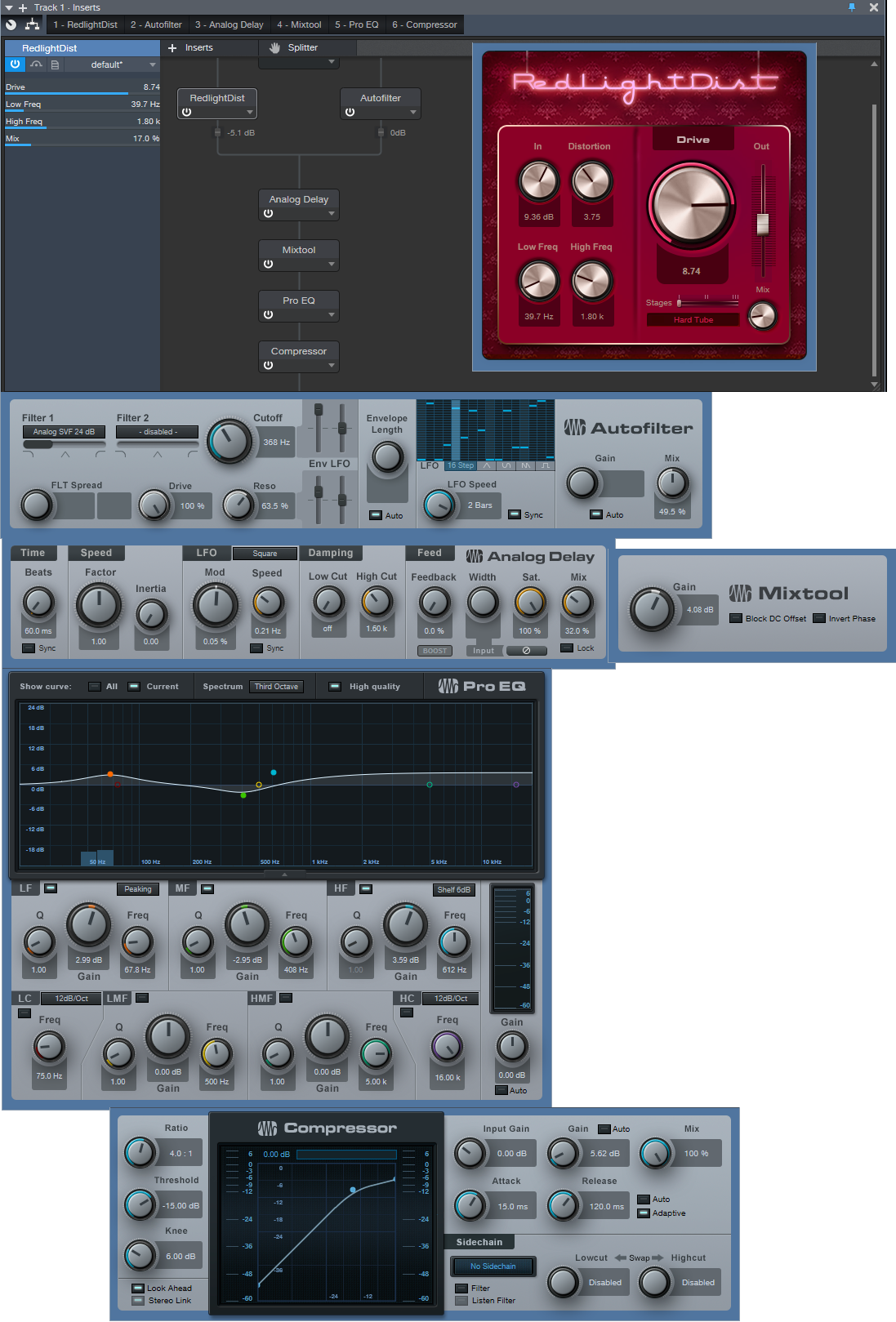
Rather than go through all the backstory on how it’s done, just download the FX Chain, and reverse-engineer it to your heart’s content. Here are the highlights, along with crucial controls you can customize to make the chain your own.

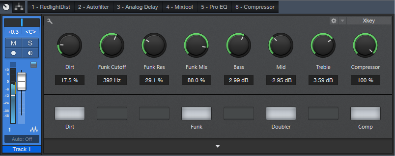
Dirt Control: This is the Mix control for the RedLightDist processor, whose settings have been optimized for bass. For more highs, turn up the processor’s High Freq control, or turn down for a bassier growl. This stage has an associated enable/bypass button.

Funk Cutoff, Funk Res, and Funk Mix: These are the essential Autofilter controls for when you want to lay some funk on your bass. Cutoff covers the general range to match your playing, Res is the filter resonance, and because envelope filters are best for bass when placed in the parallel, Mix controls the dry/filter balance. It has an associated enable/bypass switch.

Note that the RedLightDist and Autofilter are fed off a split, so they do parallel processing. This is in addition to the parallel processing done within the processors themselves.

Bass, Mid, and Treble: This “tone stack” for the Bass QuickStrip controls parameters in the Pro EQ. They don’t cover the full boost/cut range, but if you want to get more extreme, be my guest.

Compressor: The compression is optimized for bass, so the single control is a dry/compressed mix, paired with an enable/bypass switch. Any customization would be to taste—for example, a lower Threshold, or higher Ratio, for a more compressed sound. But if you want more variation and the ability to change the compression from light to heavy, another option is to use the settings for the EZ Squeez one-knob compressor, which was the subject of the Friday tip for August 24, 2018.

Doubler: This switch brings in a doubling effect, courtesy of the Analog Delay. It also bumps up the gain a bit using the Mixtool, so that the doubled and dry sounds have the same apparent level.

So download away—and lay down the low.

DOWNLOAD THE BASS QUICKSTRIP HERE! 

[Announcement: the follow-up book to “How to Record and Mix Great Vocals in Studio One” is now available—hop on over to the PreSonus Shop to check out “More than Compressors: The Complete Guide to Dynamics in Studio One.” Thank you! We now return to our regularly scheduled programming.]

Pop quiz: How many EQ plug-ins ship with Studio One Pro?

If you answered seven, congratulations! Then you know about the Pro EQ, the three different Fat Channel EQs, Ampire’s Graphic Equalizer, the Channel Strip, and using the Multiband Dynamics as a really hip graphic EQ. But actually, the correct answer is eight.

If you turn off the “auto” aspects of the Autofilter, you can take advantage of two filters, each with multiple filter topologies: three “rhymes-with-vogue”-style lowpass Ladder filters (sorry, if I mention the actual synthesizer name, I get hassled), two analog state-variable filters (yes, the same topology as the infamous Project #17, the “Super Tone Control,” in my book Electronic Projects for Musicians), one digital state-variable filter, a comb filter, and a zero-delay, 24/dB octave low-pass filter. Furthermore, you can route the two filters in series, or in parallel, as well as offset their cutoff frequencies from each other by up to 2 octaves.

The state-variable filters are particularly interesting because you can alter the response continuously from lowpass, to bandpass, to highpass, all with variable cutoff and resonance. This gives responses that are difficult, if not impossible, to obtain any other way.
So who cares about different filter types, anyway—other than guitar players who want to get totally rad wah effects? Well, these are invaluable for sound design, FX and breaks for DJs, synthesizer sweeps, and to add spice to tracks that sound just too darn normal. Don’t think of these filters necessarily as standard EQ, but more like EQ-based special effects. These parameters are automatable too, which opens up even more possibilities.

Using the testing procedure described in the Testing, Testing tip from May 16, let’s look at some of the spectral responses this exceptionally versatile pair of filters can produce.

But First, Turn Off Everything that Says Auto

To use the Autofilter as a filter, we need to turn off the automated aspects. Ctrl+click on both pairs of Env and LFO sliders to zero them out. Now we’re left with only the filters, not the modulators trying to control them. Also turn off the gain’s Auto function, because in some of the unusual ways we’ll be using the filter, overloading and nasty distortion can result from Auto gain.

Filtering Time

Fig. 1 shows the response for the 24 dB/octave ladder filter, with resonance turned up. Note that the Pro EQ high cut (lowpass) and low cut (highpass) filters can’t create this kind of curve, because they don’t have resonance controls. This is very much like the response of the classic rhymes-with-“vogue” filter, and you can automate the filter cutoff for grandiose filter sweeps.

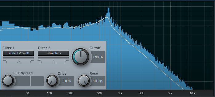
Figure 1: 24/dB ladder response, with resonance.

But wait! There’s more—because there are two different filter sections, you can offset the resonant frequencies to create double peaks. In Fig. 2, the frequencies are offset by two octaves, and the filters are in parallel (see the section outlined in orange). So now we have a double-peak ladder filter…cool.

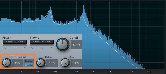
Figure 2: Double-peak ladder filter.

We can also do the “twin peaks” type of filter effect with the state-variable filters set to bandpass mode (Fig. 3). Here the filters are in parallel, and as with the above curve, they’re offset two octaves apart.

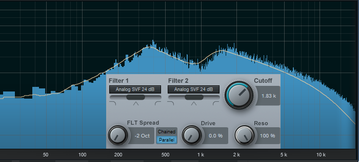
Figure 3: Dual bandpass filters in parallel can create twin peak filter responses, with fairly steep “skirts” on both sides of the peaks.

If you chain the two state-variable filters in series, set them to bandpass mode, don’t offset them, and boost the resonance, the filter curve makes a wonderful wah pedal (Fig. 4). The peak is sharp, with a steep rolloff on either side.

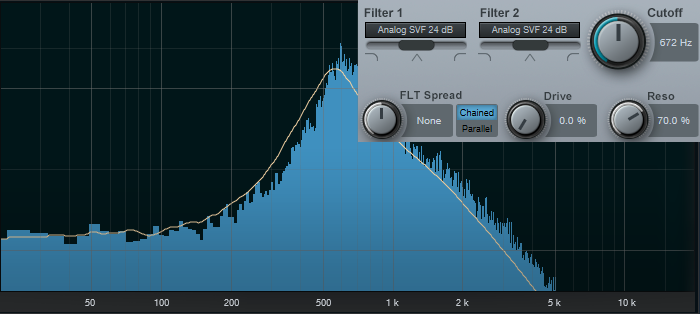
Figure 4: If you’re looking for a wah pedal sound…start here.

This also produces a strong sense of pitch with white or pink noise. One cool trick is using this setting to add a “tuned” aspect to snare drums, and other percussion instruments. Edit Studio One’s Tone Generator plug-in to generate pink noise, feed that into the above filter configuration, turn up the resonance, tune the cutoff to the desired pitch, then gate the noise with a snare hit. Mix in the desired amount of noise to give the drum a sense of pitch.

The highpass setting is useful as well, because you can obtain what’s popularly called the “voice of the Gods” effect for announcing and narration. Using a highpass filter gets rid of the super-low-frequency p-pops, but the resonance adds a boost in the bass range above the nasty stuff, so the voice still sounds full and big (Fig. 5).

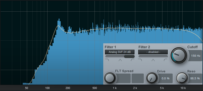
Figure 5: A high-pass filter with resonance can do wonders for narration.

It’s also possible to create responses that are just plain unusual, like this notch + double peak outside of the notch (Fig. 6). For some sound-design type wind sounds, drop the resonance to around 30%, and sweep the cutoff between 2 kHz and 6 kHz. Modulating randomly around a relatively low cutoff frequency can also give good rain and downpour sounds. Besides, who doesn’t like a curve that looks like Batman.

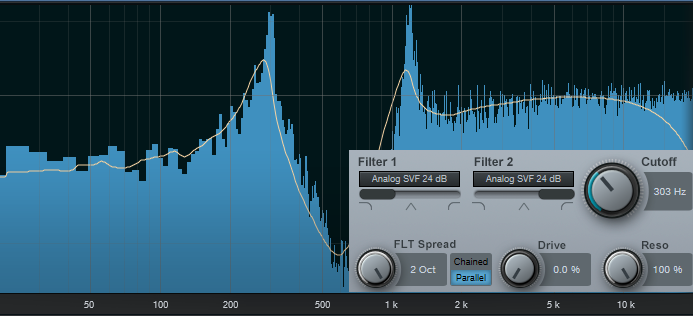
Figure 6: This unusual filter response has various uses for sound design.

Combining two different filter topologies can also give interesting results. Fig. 7 shows a ladder filter in parallel with a state variable filter, along with considerable amounts of resonance. If you really want to scope out this configuration’s flexibility, vary the Filter 2 slider to alter the topology, and/or vary the Filter Spread to change the offset between the two filter types. Of course, changing resonance alters the sound even further.

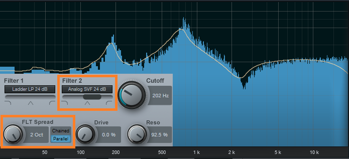
Figure 7: This filter configuration is in love with sound design and automation.

And finally…this is going to sound ridiculous, but bear with me. I often augment sampled female choir presets; octave lower sine waves mixed in subtly can give the illusion of a male choir combined with a female choir. But that’s not all—noise can be a powerful enhancer for choirs, and it’s possible to set the Autofilter to impart vocal-like qualities to pink noise.

For this application, the Zero Delay LP 24 dB is the filter of choice to insert after the Tone Generator’s pink noise output, because the filtering has a smooth kind of quality, even with high resonance. To concentrate the spectrum on voice, a Pro EQ follows the Autofilter to take off the highs and lows outside of the vocal range (Fig. 8).

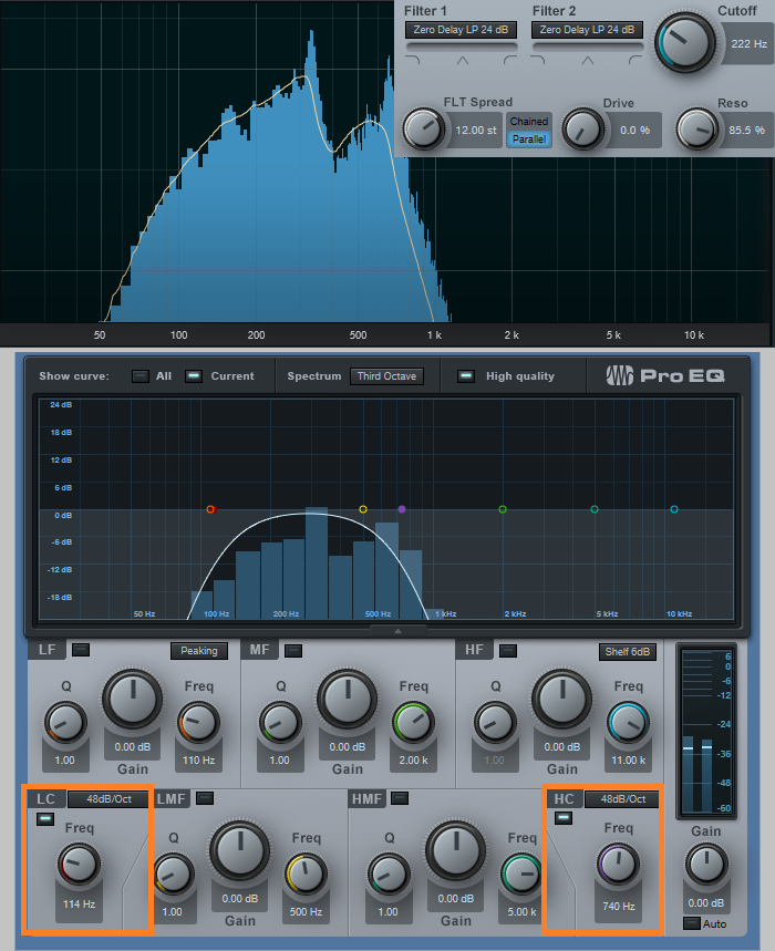
Figure 8: The Pro EQ shapes the pink noise into more of the vocal range.

Okay, now for the bummer: You can’t control the Autofilter cutoff, and therefore the pitch, with notes—only controllers. That’s not a problem if you just need a kind of pedal point choir addition; tune the cutoff to the desired pitch, and use volume automation to bring it in and out.

One workaround is to sample the resulting choir-like noise at different pitches, and load them into Sample One XT (or Impact XT) so you can create envelopes that match the envelope of whatever choir sound you’re using, and play the notes from a keyboard. The result is uncanny—in some ways, it makes a sampled choir sound more like a real choir than if it consisted only of samples. And finally, for sound design, don’t forget that filtered white noise can also augment crowd sounds.

Autofilter? Okay, yeah, well…I guess. But there’s a lot more to the story than just wah pedals and funk bass.

Grab a copy of Craig’s latest eBook here! 

Sure, everyone sorta knows about saturation. But let’s drill down, give some audio examples that really get the point across, and explain how saturation can help everything from individual tracks to master tapes. Really.

To be clear, we’re not talking about the distortion that “flat-tops” a waveform. Fig. 1 shows a comparison of unsaturated, saturated, and distorted versions of the same waveform (using version 4.5’s new “smooth” waveform view feature).

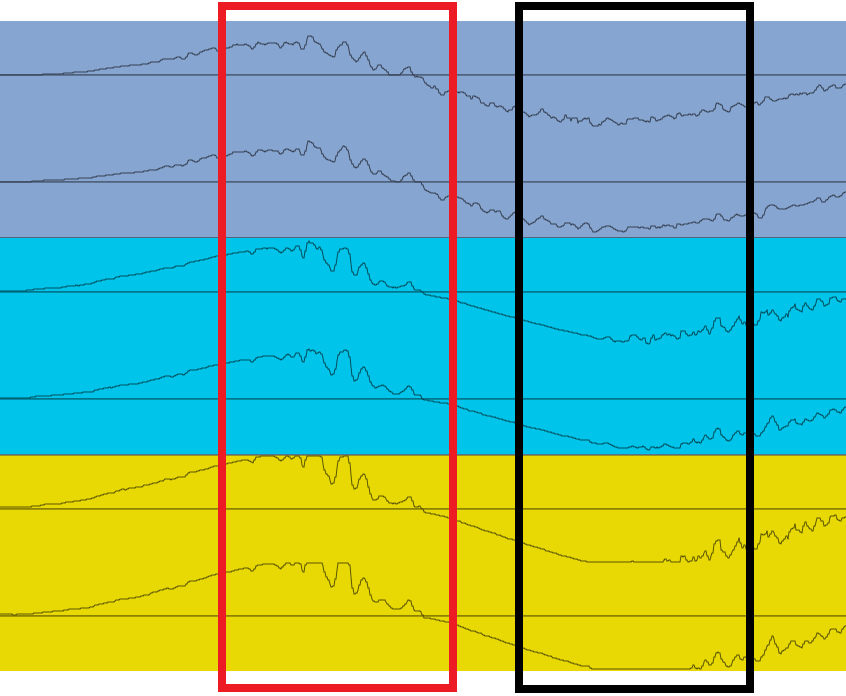
Figure 1: The gray waveform is unsaturated, the blue saturated, and the yellow distorted.

Comparing the three, in the section outlined in red, the saturated version is louder but the waveform isn’t all that different from the unsaturated audio. The distorted waveform is louder than the saturated one, but the peaks are flattened. This is particularly noticeable with the negative-going peak highlighted in black. Flattening peaks produces the kind of nasty digital distortion no one really likes, but saturation is a different animal…as the audio examples will show.

Before going any further, if you don’t have the free Softube Saturation knob, go to your PreSonus account and download it from Products > Add-Ons (Fig. 2).

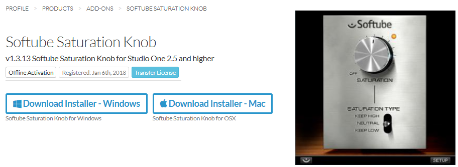
Figure 2: What are you waiting for? It’s free.

It’s a pretty basic module—turn the knob clockwise for more saturation (but I’ve never turned it up as high as shown in the picture!). Keep Low means it will apply more saturation to high frequencies, Keep High means more saturation for low frequencies, and Neutral means equal-opportunity saturation for all frequencies.

Saturation is great with drums, including mixed drums. You’ll get more punch and level (Fig. 3) that helps drums stand out in a track, without any of the artifacts (like pumping or breathing) associated with some dynamics processors.

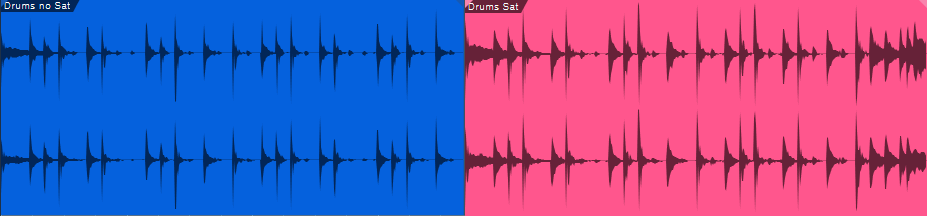
Figure 3: The waveform for the drums audio example. Unsaturated is blue, saturated is red.

Now listen to the audio example. The first four measures are the unsaturated version, the last four measures the saturated one. Note that both were normalized to the same peak value. Even though the waveforms don’t look all that different, the saturated version really punches through—yet doesn’t sound “distorted.” This same kind of approach can also work well for bass.

 Now, let’s move on to saturating a two-track master. This may sound like a bad idea, until you realize that tape emulation plug-ins are basically just adding saturation, although some do it with a bit more finesse than a simple saturation plug-in (e.g., the Waves J37 provides different virtual tape formulations and bias settings). Fig. 4 shows the audio example’s waveform.

Figure 4: The two blue, four-measure groups are unsaturated; the two red, four-measure groups are saturated.

The audio example is excerpted/adapted from the song All Over Again (Every Day). I added a very slight pause between the unsaturated and saturated sections, although I’m quite sure you’ll hear the difference anyway. (To hear the final, mastered song—which of course was done in Studio One—click on the link.)

For this kind of application, you don’t want to apply too much saturation—a little bit goes a long way. As you turn up the knob you may think it’s not really making a difference, but it is. Toggle bypass frequently for a reality check. Fig. 5 shows the settings used for the master tape example.

And there you have it—we’ve done our shoutout for saturation. If you’ve missed out on the fun, load it in a track, and listen to what happens. You just might like what you hear!

I like anything that kickstarts creativity and gets you out of a rut—which is what this tip is all about. And, there’s even a bonus tip about how to create a Macro to make this process as simple as invoking a key command.

Here’s the premise. You have a MIDI drum part. It’s fine, but you want to add interest with a fill in various measures. So you move hits around to create a fill, but then you realize you want fills in quite a few places…and maybe you tend to fall into doing the same kind of fills, so you want some fresh ideas.

Here’s the solution: Studio One 4.5’s new Randomize menu, which can introduce random variations in velocity, note length, and other parameters. But what’s of interest for this application is the way Shuffle can move notes around on the timeline, while retaining the same pitch. This is great for drum parts.

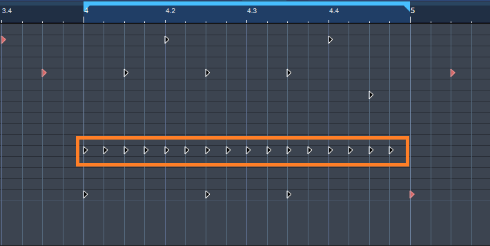
The following drum part has a really simple pattern in measure 4—let’s spice it up. The notes follow an 8th note rhythm; applying shuffle will retain the 8th note rhythm, but let’s suppose you want to shuffle the fills into 16th-note rhythms.

Here’s a cool trick for altering the rhythm. If you’re using Impact, mute a drum you’re not using, and enter a string of 16th notes for that drum (outlined in orange in the following image). Then select all the notes you want to shuffle.

Go to the Action menu, and under Process, choose Randomize Notes. Next, click the box for Shuffle notes (outlined in orange).

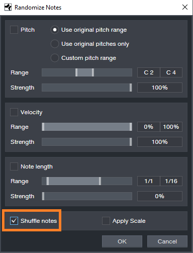
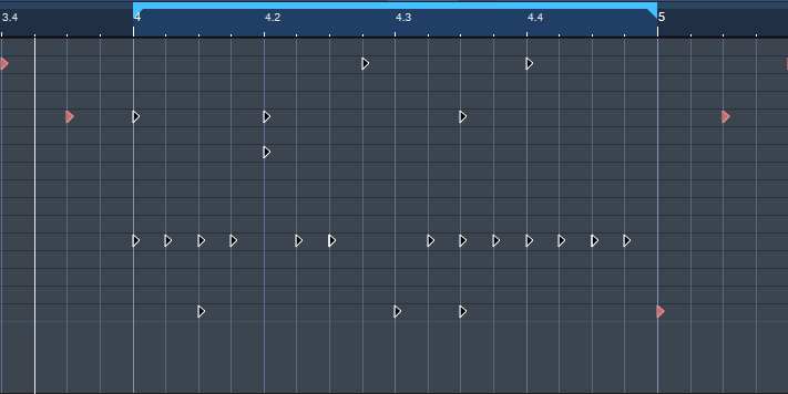
Click on OK, and the notes will be shuffled to create a new pattern. You won’t hear the “ghost” 16th notes triggering the silent drum, but they’ll affect the shuffle. Here’s the pattern after shuffling.

If you like what you hear from the randomization, great. But if not, adding a couple more hits manually might do what you need. However, you can also make the randomizing process really efficient by creating a Macro to Undo/Shuffle/hit Enter.

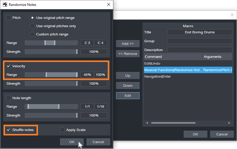
Create the Macro by clicking on Edit|Undo in the left column, and then choose Add. Next, add Musical Functions|Randomize. For the Argument, check Shuffle notes; I also like to randomize Velocity between 40% and 100%. The last step in the Macro is Navigation|Enter. Finally, assign the Macro to a keyboard shortcut. I assigned it to Ctrl+Alt+E (as in, End Boring Drum Parts).

With the Macro, if you don’t like the results of the shuffle, then just hit the keyboard shortcut to initiate another shuffle…listen, decide, repeat as needed. (Note that you need to do the first in a series of shuffles manually because the Macro starts with an Undo command.) It usually doesn’t take too many tries to come up with something cool, or that with minimum modifications will do what you want. Once you have a fill you like, you can erase the ghost notes.

If the fill isn’t “dense” enough, no problem. Just add some extra kick, snare, etc. hits, do the first Randomize process, and then keep hitting the Macro keyboard shortcut until you hear a fill you like. Sometimes, drum hits will end up on the same note—this can actually be useful, by adding unanticipated dynamics.

Perhaps this sounds too good to be true, but try it. It’s never been easier to generate a bunch of fills—and then keep the ones you like best.

Studio One has several analysis tools, and you can use them to learn a lot about how effects work. One of my favorite test setups is inserting the Tone Generator at the beginning of the Insert Device Rack to generate white noise (a test signal with equal energy throughout the audio spectrum), the Spectrum Meter at the end of the Rack, and the device under test in between them. Here’s the Tone Generator, set to generate white noise.

As one example of the benefits of testing gear, a lot of engineers like the gentle tone-shaping qualities of Pultec’s MEQ-5 midrange equalizer. So you need an MEQ-5 plug-in, or the hardware, to obtain that effect with Studio One…right? Maybe not.

One reason for the “sound” of Pultec equalizers is that they used passive circuitry, so the EQ curves were broad. But the Pro EQ can do gentle curves as well, simply by choosing a low Q setting. The screen shot shows Pro EQ settings for a “Pultec-like” curve, with a considerable amount of boost and cut.

But how much is it really like a Pultec? Let’s find out. Choose the same settings on the Pro EQ and on an MEQ-5, then run some white noise through both, using the Spectrum Meter’s FFT analysis.

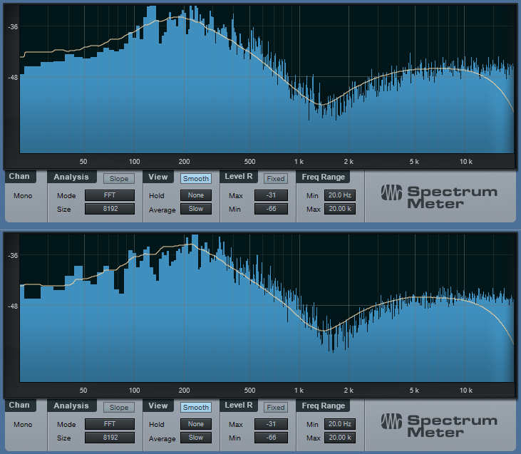
The white, smoothed line shows the average frequency response (white noise is changing constantly because it’s random, so in this case we want a smoothed, average reading). The top graph is the Pro EQ, and the bottom graph is the MEQ-5. Sure, there may be some subtle sonic differences due to the use of different filter topologies. But if you’re looking for those gentle, tone-shaping curves, the Pro EQ does just fine.

You can also find out exactly what’s going on with some effects. For example, Studio One has a phase shifter effect, and you probably know that phase shifting produces notches in the audio. But how deep are the notches? And how far apart are they? Let’s take a look.

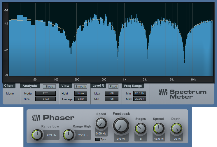
The Phaser is set to 8 stages, so there are 4 notches. For this measurement, we want to know the instantaneous value of the notches, so the average isn’t smoothed. With depth up full, the notches are around -35 dB or so.

While we’re at it, let’s check the frequency response of guitar cabinets, so we can find out why they sound so different from each other.

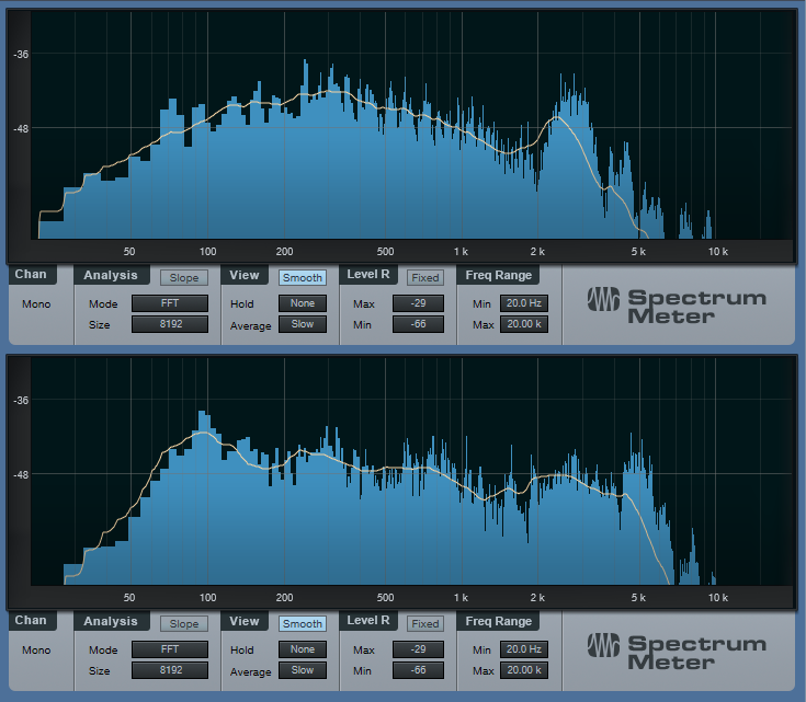
The upper image shows the response for a Mesa Boogie Mark IV cabinet. Note the prominent peak in the 3 kHz range, and the rolloff below 200 Hz—now you know why those solos can really cut through a mix. Compare that with the lower image of a 1965 Fender Princeton. It has a low end bump to give a full sound, a bit of a notch around 1.5 kHz, and has more high end above 5 kHz than the Mark IV.

As to why these readings matter, suppose you recorded a guitar part, and want it to have more of a Mesa Boogie vibe. Just tweak your EQ accordingly to approximate the curve.

Using white noise for testing can also show why SSL E-series and G-series EQ curves are different, the differences between standard and constant-Q parametric stages, what really happens when you move graphic EQ sliders around, and more. If you’re curious about scratching beneath the GUI of your effects, Studio One’s analysis tools can reveal quite a bit.