Category Archives: Studio One
Make Bass “Pop” in Your Mix
Bass has a tough gig. Speakers have a hard time reproducing such low frequencies. Also, the ear is less sensitive to low (and high) frequencies compared to midrange frequencies. Making bass “pop” in a mix, especially at low playback levels, isn’t easy.
Fortunately, saturating the bass can provide a solution. This type of distortion has two beneficial effects:
- Adds high-frequency harmonics. A bass note with harmonics is easier to hear, even in systems with a compromised bass response and at lower playback levels.
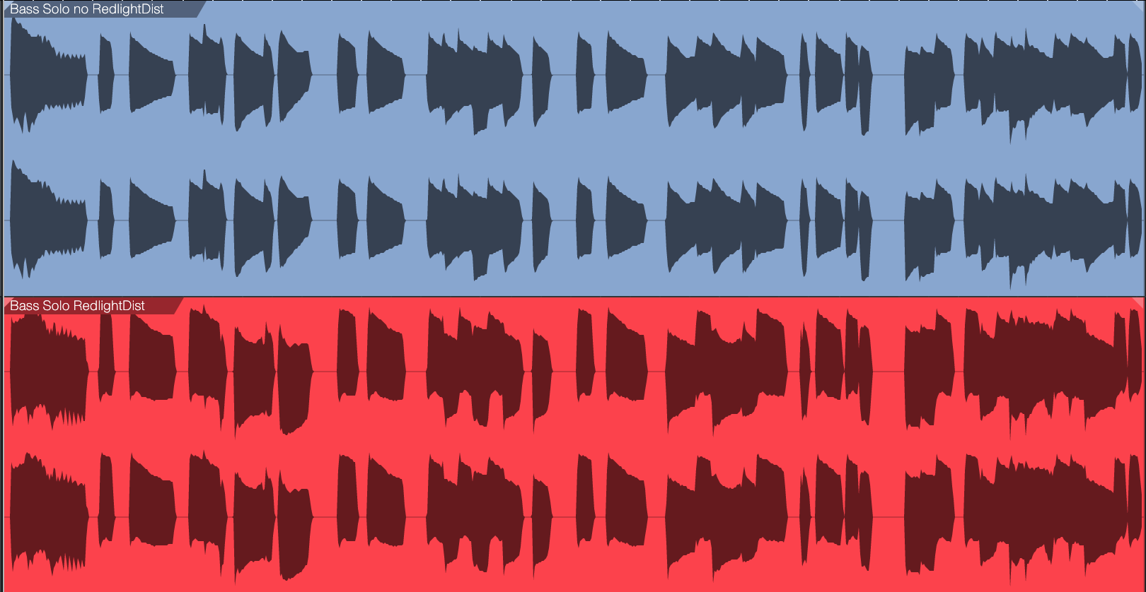
- Raises the bass’s average level. With light saturation, the bass has a higher average level. But this doesn’t have to increase the peak level (fig. 1).
Most bass lines use single notes. So, unlike guitar, saturation doesn’t create nasty intermodulation distortion due to notes interacting with each other. Even with saturation, the bass sounds “clean” in the context of a mix.
The Star of the Show: RedlightDist
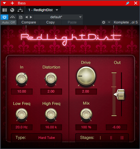
Although tape emulation effects are popular for saturating bass, RedlightDist (fig. 2) is all you need. Setting Type to Hard Tube and using a single Stage produces an effect with bass that’s almost indistinguishable from tape emulation plugins. (The Bass QuickStrip tip also includes the RedlightDist, but the preset uses the Splitter. This simpler tip works with Studio One Artist or Professional.)
How to Optimize the Input Level
The saturation amount depends on the input level, not just the settings of the In, Distortion, and Drive controls. The Distortion and Drive settings in fig. 2 work well. At least initially, use the In control to adjust the amount of saturation. If the highest setting doesn’t produce enough saturation, increase the level going into the RedlightDist. If you still want more saturation, increase Drive.
Hearing is Believing!
Make sure you check out these audio examples, because the way RedlightDist affects the overall mix is dramatic. First, listen to the unprocessed bass sound as a reference. All the examples are normalized to ‑6 dB peak levels.
The next example is the saturated sound. But the real payoff is in the final two examples.
The following example plays an excerpt from a song. The bass is not saturated. Listen to it in context with the mix.
The final example uses saturated bass in the song excerpt. Listen to how the bass stands out in the mix, even though its peak level is the same as the previous example.
By using saturation, you can mix the bass lower than you could without saturation, yet the bass sounds equally prominent. This offers two main benefits:
- There’s more low-frequency space for the kick and other instruments.
- Having less low-bass energy frees up more headroom. So, the entire mix can have a higher level, without needing to add compression or limiting.
RedlightDist is a versatile effect. Also try this technique with kick—as well as analog, beatbox-style drum sounds—when you need more punch and pop.
Enhance Your Reverb’s Image
First, an announcement: If you own the eBook “How to Record and Mix Great Vocals in Studio One,” you can download the 2.1 update for free from your PreSonus account. This new version, with 10 chapters and over 200 pages, includes the latest features in Studio One 6. New customers can purchase the eBook from the PreSonus Shop. And now, this week’s tip…
Studio One’s Room Reverb creates realistic ambiance, but sometimes “realistic” isn’t the goal. Widening the reverb’s stereo image outward can give more clarity to sounds panned to center, such as kick, snare, and vocals. Expanding the image also gives a greater sense of width.
This tip covers four ways to widen the reverb’s image. All these techniques insert reverb in an FX Channel. The channels you want to process with reverb feed the FX Channel via Send controls.
#1 Easiest Option: Binaural Pan
Version 6 upgraded the mixer’s panpot to do dual panning or binaural panning, in addition to the traditional balance control function. Click on the panpot, select Binaural from the drop-down menu, and turn up the Width control to widen the stereo image (fig. 1).
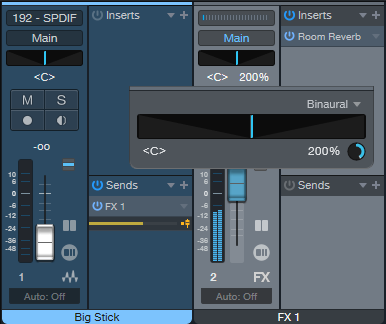
If you haven’t upgraded to version 6 yet, then insert the Binaural Pan plug-in after the reverb. Turn up the Binaural Pan’s Width parameter for the same widening effect.
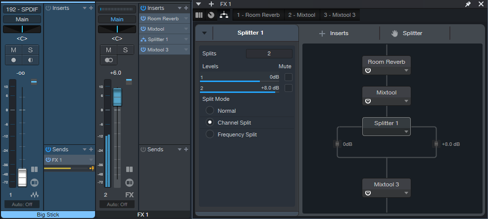
#2 Most Flexible: Mid-Side Processing
Mid-side processing separates the mid (center) and side (left and right) audio. (For more about mid-side processing, see Mid-Side Processing Made Easy and Ultra-Easy Mid-Side Processing with Artist.) The advantage compared to the Binaural Pan is that you can process the sides or center audio, as well as adjust their levels. This tip uses the Splitter module in Studio One Professional.
In fig. 2, the Room Reverb feeds a Mixtool. Enabling the Mixtool’s MS Transform function encodes stereo audio so that the mid audio appears on the left channel, and the sides audio on the right. The Splitter is in Channel Split mode, so its Level parameters set the levels for the mid audio (Level 1) and sides audio (Level 2). To widen the stereo effect, set Level 2 higher than Level 1. The final Mixtool, also with MS Transform enabled, decodes the signal back into conventional stereo.
#3 Most Natural-Sounding: Dual Reverbs and Pre-Delay
This setup requires two FX Channels, each with a reverb inserted (fig. 3).
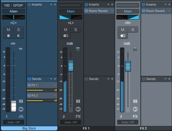
To create the widening effect:
1. Edit one reverb for the sound you want.
2. Pan its associated FX Channel full left.
3. Copy the reverb into the other channel, and pan its associated FX Channel full right.
4. To widen the stereo image, increase or decrease the pre-delay for one of the reverbs. The sound will be similar to the conventional reverb sound, but with a somewhat wider, yet natural-sounding, stereo image.
Generally, copying audio to two channels and delaying one of them to create a pseudo-doubling effect can be problematic. This is because collapsing a mix to mono thins the sound due to phase cancellation issues. However, the audio generated by reverb is diffuse enough that collapsing to mono doesn’t affect the sound quality much (if at all).
#4 Most Dramatic: Dual Reverbs with Different Algorithms
This provides a different and dramatic sense of width. Use the same setup as the previous tip, but don’t increase the pre-delay on one of the reverbs. Instead, change the Type algorithm (fig. 4).
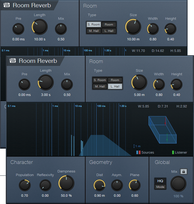
If you change one of the reverbs to a smaller room size, you’ll probably need to increase the Size and Length to provide a balance with the reverb that has a bigger room size. Conversely, if you change the algorithm to a larger room, decrease Size and Length. You may also need to vary the FX Channel levels if the stereo image tilts to one side.
Free! Three Primo Piano Presets
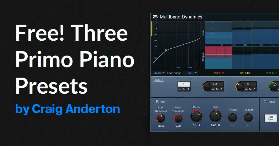
Let’s transform your acoustic piano instrument sounds—with effects that showcase the power of Multiband Dynamics. Choose from two download links at the end of this post:
- FX Chains. These include the FX part of the Instrument+FX Presets (see next), so you can use them with any acoustic piano virtual instrument. You may want to bypass any effects added to the instrument (if present) so that the FX Chains have their full intended effect. Then, you can try adding the effects back in to see if they improve the sound further.
- Instrument+FX Presets. These are based on the PreSonus Studio Grand piano SoundSet. This SoundSet comes with a Sphere membership, or is optional-at-extra-cost for Studio One Artist or Professional.
Remember, presets that incorporate dynamics will sound as intended only with suitable input levels. These presets are designed for relatively high input levels, short of distortion. If the presets don’t seem to have any effect, increase the piano’s output level. Or, add a Mixtool between the channel input and first effect to increase the level feeding the chain.
CA Studio Grand Beautiful Concert
Before going into too different a direction, let’s create a gorgeous solo piano sound. In this preset, the Multiband Dynamics has two functions. The Low band compresses frequencies below 100 Hz (fig. 1), to increase the low end’s power.
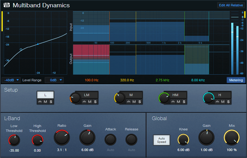
The HM stage is active, but doesn’t compress. It acts solely as EQ. By providing an 8 dB boost from 2.75 kHz to 8 kHz, this stage adds definition and “air.” The remaining effects include Room Reverb for ambiance and Binaural Pan to widen the instrument’s stereo image. Let’s listen to some Debussy.
CA Studio Grand Funky
Although not intended as an emulation, this preset is inspired by the punchy, funky tone of the Wurlitzer electric pianos produced from the 50s to the 80s. The Multiband Dynamics processor solos, and then compresses, the frequency range from 250 Hz to 9 kHz (fig. 2).
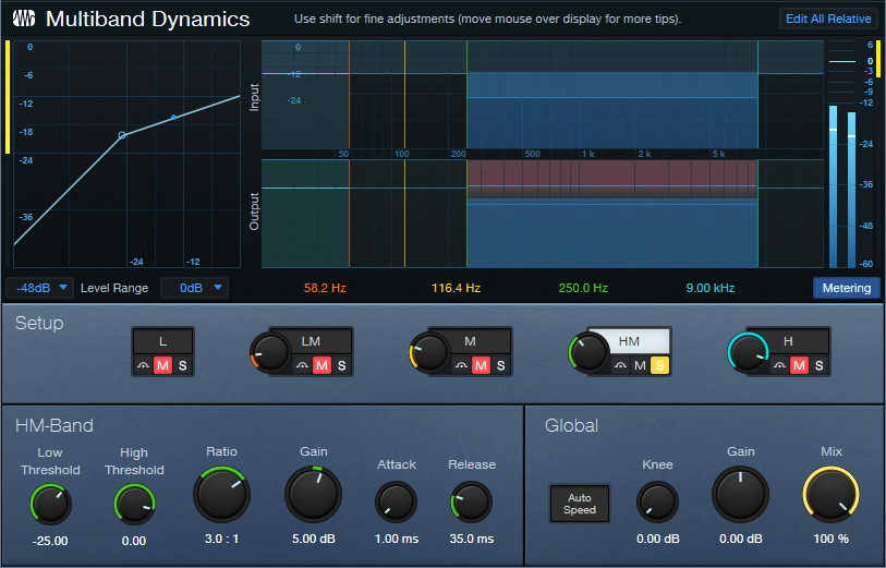
The post-instrument effects include a Pro EQ3 to impart some “honk” around 1.6 kHz, and the RedlightDist for mild saturation. X-Trem is optional for adding vintage tremolo FX (the audio example includes X-Trem).
CA Studio Grand Smooth
This smooth, thick piano sound is ideal when you want the piano to be present, but not overbearing. The Multiband Dynamics has only one function: provide fluid compression from 320 Hz to 3.50 kHz (fig. 3). This covers the piano’s “meat,” while leaving the high and low frequencies alone.
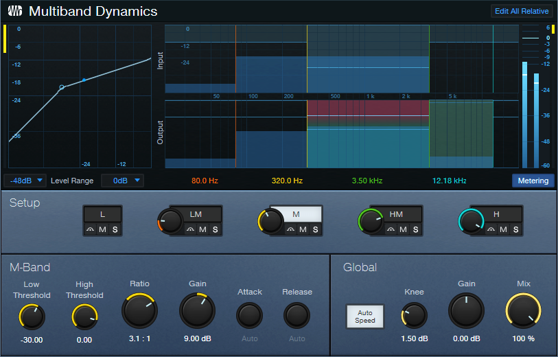
The audio example highlights how the compression increases sustain on held notes.
Hey—Up for More?
These presets just scratch the surface of how multiband dynamics and other processors can transform instrument sounds. Would you like more free instrument presets in the future? Let me know in the comments section below.
Download the Instrument+FX Presets here:
Download the FX Chains here:
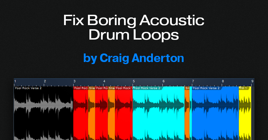
Fix Boring Acoustic Drum Loops
Acoustic drum loops freeze-dry a drummer’s playing—so, what you hear is what you get. What you get. What you get. What you get. What you get. What you get.
Acoustic drums played by humans are inherently expressive:
- Human drummers don’t play the same hits exactly the same way twice.
- Drummers play with subtlety. Not all the time, of course. But ghost notes, dynamic extremes, and slight timing shifts are all in the drummer’s toolkit.
Repetitive loops cue listeners that a drum part has been constructed, not played. So, let’s explore techniques that make acoustic drum loops livelier and more credible. (We’ll cover tips for MIDI drums in a future post.)
Loop Rearrangement
Simply shuffling a few of a loop’s hits within a loop may be all that’s needed to add interest. The following audio examples use a looped verse, and a fill, from Studio One’s Sound Sets > Acoustic Drum Kits and Loops > Fool Rock > Verse 132 BPM.
The first clip plays the Fool Rock Verse 2 loop four times (8 measures), without changes. It quickly wears out its welcome.
We can improve the loop simply by shuffling one snare hit, and adding part of a fill (fig. 1).
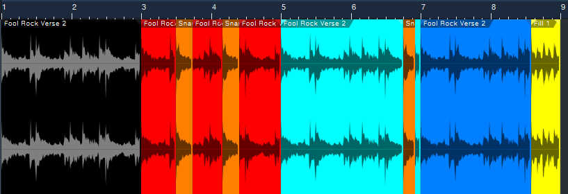
The black loop at the beginning is the original two-measure loop. It repeats three more times, although there are some changes. The red loop is the same, except that a copy of its first snare hit (colored orange) replaces a kick hit later in the loop.
The light blue loop uses the same orange snare hit to provide an accent just before the loop’s end. The copied snare sounds different from the snare that preceded it, which also increases realism.
The dark blue loop is the same as the original, except that it adds the last half of the file Fool Rock Fill 1 at the end.
Listen to how even these minor changes enhance the drum part.
Cymbal Protocol
The Fool Rock folder has two different versions of the Verse 2 loop. One has a crash at the beginning, one doesn’t. I’m not a fan of loops with a cymbal on the first beat. With loops that are only two measures long, repeating the loop with the cymbal results in too many cymbals for my taste. Besides, drummers don’t use cymbals just to mark the downbeat, but to add off-beat hits and accents.
The loops in fig. 1 use the version without a crash. If we replace the first loop with the version that has a crash, the cymbal doesn’t become annoying because it’s followed by three crashless loops. But it’s even better if you overdub cymbals to add accents.
The final audio clip’s first two measures use the Fool Rock loop that includes a crash on the downbeat. However, there are now two cymbal tracks in addition to the loop. A hit from each cymbal creates a transition between the end of the second loop, and the beginning of the third loop.
Loop Ebb and Flow
In this kind of 8-measure figure with 2-measure loops, it’s common for the first and third loops to be similar or even identical. The second loop will add some variations, and the fourth loop will have a major variation at the end to “wrap up” the figure. This natural ebb and flow mimics how many drummers create parts that “breathe.” Keep this in mind as you strive for more vibrant, life-like drum parts.
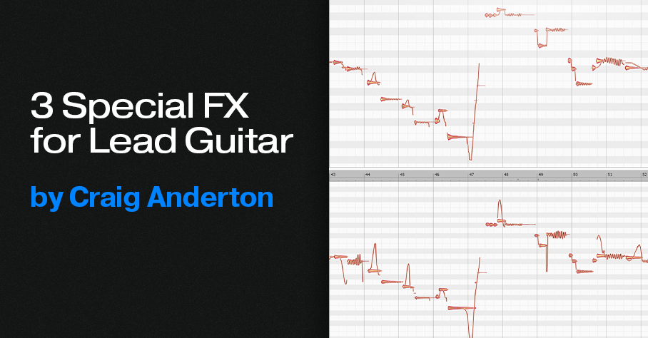
3 Special FX for Lead Guitar
Melodyne can do much more than vocal pitch correction. Previous tips have covered how to do envelope-controlled flanging and polyphonic guitar-to-MIDI conversion with Melodyne Essential. The following techniques add mind-bending effects to lead guitar, and don’t involve pitch correction per se.
However, all three tips require the Pitch Modulation and Pitch Drift tools. These tools are available only in versions above Essential (Assistant, Editor, and Studio). A Melodyne 5 trial version incorporates these versions. The trial period is 30 days, during which there are no operational limitations.
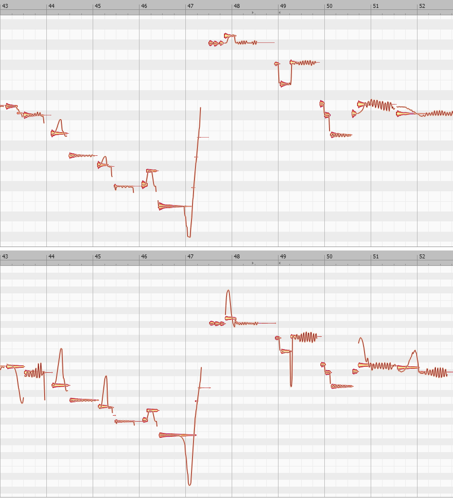
Fig. 1 shows a lead guitar line, before and after processing, that incorporates all three processing techniques. This is the melody line used in the before-and-after audio example.
Vibrato Emphasis/De-Emphasis
To increase or decrease the vibrato amount, use Melodyne’s Pitch Modulation tool. In fig. 1, the increased vibrato effect is most visually obvious at the end of measures 43, 49, and 52. To change the amount of vibrato, click on the blob with the Pitch Modulation tool. While holding the mouse button down, drag up (more vibrato) or down (less vibrato). Extreme vibrato amounts can sound like whammy bar-based vibrato.
Synthesized Slides
Notes with moderate bending can bend pitch up or down over as much as several semitones:
1. Select the Pitch Modulation tool.
2. Click on a blob that incorporates a moderate bend.
3. While holding the mouse button down, drag up to increase the bend up range. With most notes, you can invert the bend by dragging down.
Because a synthesized bend can cover a wider pitch range than physical strings, this effect sounds like you’re using a slide on your finger. In fig. 1, see measures 44 and 45 for examples of upward bends. The end of measure 47 shows an increased downward bend.
For the most predictable results, the note you want to bend should:
- Establish its pitch before you start bending. If you start a note with a bend, Melodyne may think the bent pitch is the correct one. This complicates increasing the amount of bend.
- Have silence (however brief) before the note starts. If there’s no silence, before opening the track in Melodyne, edit the guitar track to create a short silent space before the note.
Slide Up to Pitch, or Slide Down to Pitch
This is an unpredictable technique, but when it works, note transitions acquire a “smooth” character. In fig. 1, note the difference between the modified and unmodified pitch slides in measures 43, 44, 47, 49, 50, and 51.
To add this kind of slide, click on a blob with the Pitch Drift tool, and then drag up or down. The slide’s character depends on what happens during, before, and after the note. Sometimes using Pitch Modulation to initiate a slide, and Pitch Drift to modify the slide further, works best. Sometimes the reverse is true.
This is a trial-and-error process. With experience, you’ll be able to recognize which blobs are good candidates for slides.
The ”Hearing is Believing” Audio Examples
Guitar Solo.mp3 is an isolated guitar solo that uses none of these techniques.
Guitar Solo with Melodyne.mp3 uses all of these techniques on various notes.
To hear these techniques in a musical context that shows how they can add a surprising amount of emotion to a track,this link takes you to a guitar solo in one of my songs on YouTube. The solo uses all three effects.
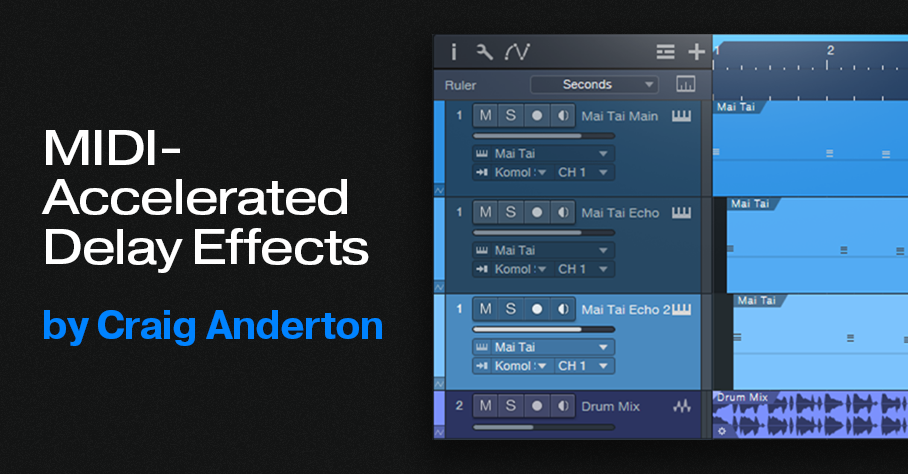
MIDI-Accelerated Delay Effects
Synchronized echo effects, particularly dotted eighth-note delays (i.e., intervals of three 16th notes), are common in EDM and dance music productions. The following audio example applies this type of Analog Delay effect to Mai Tai.
However, you can also create echoes for virtual instruments by copying, offsetting, and editing an instrument track’s MIDI note data. In the next audio example, the same MIDI track has been copied and delayed by an 8th note (fig. 1).
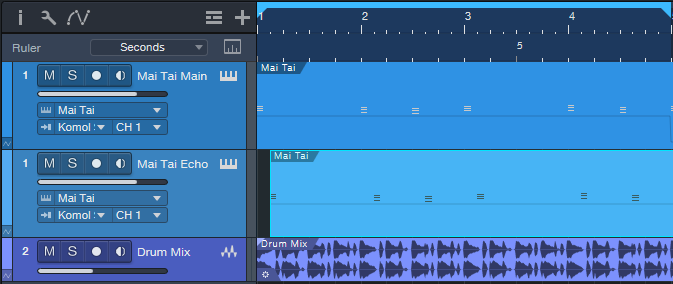
In the original instrument track, the MIDI note data velocities are around 127. These values push the filter cutoff close to maximum. Reducing the copied Echo track’s velocity to about half creates notes that don’t open up the Mai Tai’s filter as much. So, the MIDI-generated delay’s timbre is different.
The next track copies the original track again. But this time, the notes are transposed up an octave, and offset by a dotted eighth-note compared to the original (fig. 2). For this track, the velocities are about halfway from the maximum velocity.
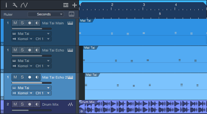
Now we have our “MIDI-accelerated” echo effect for the virtual instrument’s notes, which are still processed by the original Analog Delay effect. The final audio example highlights how the combination of analog delay and MIDI note delay evolves over 8 measures.
These audio examples are only the start of what you can do with MIDI echo by offsetting, transposing, and altering note velocities. You can even feed the different MIDI tracks into different virtual instruments, and create amazing polyrhythms. But why stop there? Hopefully, this blog post will inspire you to come up with your own signature variations on this technique.
Friday Tips in the Real World: the Sequel

This is a follow-up to the Friday Tips in the Real World blog post that appeared in 2020. It was well-received, so I figured it was time for an update.
Although many of the Friday Tips include an audio example of how a tip affects the sound, that’s different from the real-world context of a musical production. So, this blog post highlights how selected tips were used in my recent music/video project, Unconstrained. The project was recorded, mixed, and mastered entirely in Studio One.
As you might expect, the workflow-related tips were used throughout, as were some of the audio tips. For example, all the vocals used the Better Vocals with Phrase-by-Phrase Normalization technique, and all the guitar parts followed the Amp Sims: Garbage In, Garbage Out tip. The Chords Track and Project Page updates were crucial to the entire project as well.
The links take you to specific parts of the songs that showcase the tips, accompanied by links to the relevant Friday Tip blog post. If you’re curious about specific production techniques used in the project, whether they’re included in this post or not, feel free to ask questions in the comments section.
One reader’s comment for the Lead Guitar Editing Hack blog post mentioned how useful this technique is. If you missed it the first time, here’s what it sounds like applied to a solo. Attenuating the attack gives the melody line a synth-like, otherworldly sound. Incidentally, if you back up the video to 6:20, the cello sounds are from Presence. I tried the “industry standard” orchestra programs, but I liked the Presence cellos more. Also, I used the “time trap” technique from the Fun with Tempo Tracks post to slow the cellos slightly before going full tilt into the solo.
The Magic Stereo blog post described a novel way to add motion to rhythm parts, like piano and guitar. This excerpt uses that technique to move the guitar in stereo, but without conventional panning. Later on in the song, the drums use Harmonic Editing to give a sense of pitch. The post Melodify Your Beats describes this technique. But in this song, the white noise wasn’t needed because the drums had enough of a frequency range so that harmonic editing worked well.
I wrote about the EDM-style “pumping” effect in the post “Pump” Your Pads and Power Chords, and it goes most of the way through this song. The reason why I chose this section is because the solo uses Presence, which I think may be underrated by some people.
Another topic that’s dear to my heart is blues harmonica, and it loves distortion—as described in the blog post Blues Harmonic FX Chain. It’s wonderful how amp sims can turn the thin, reedy sound of a harmonica into something with so much power it’s almost like a brass section. However, note that this example uses a revised version of the original FX Chain, based on Ampire. (The revised version is described in The Huge Book of Studio One Tips and Tricks.)
The blog post Studio One’s Session Bass Player generated a lot of comments. But does the technique really work? Well, listen to this example and decide for yourself. I needed a scratch bass part but it ended up being so much like what I wanted that I made only a couple tweaks…done. For a guitar solo in the same song, I tried a bunch of wah pedals but the one that worked best was Ampire’s.
I still think Studio One’s ability to do polyphonic MIDI guitar courtesy of Melodyne (even the Essential version) is underrated. This “keyboard” part uses Mai Tai driven by MIDI guitar. The MIDI part was derived from the guitar track that’s doubling the Mai Tai. For more information, see the blog post Melodyne Essential = Polyphonic MIDI Guitar. Incidentally, except for the sampled bass and choir, all the keyboard sounds were from Mai Tai. If you’ve mostly been using third-party synths, spend some time re-acquainting yourself with Mai Tai and Presence. They can really deliver.
As the post Synthesize OpenAIR Reverb Impulses in Studio One showed, it’s easy to create your own reverb impulses for OpenAIR. In this excerpt, the female background vocals, male harmony, and harmonica solo all used impulses I created using this technique. (The only ambience on the lead vocal was the Analog Delay). Custom impulses are also used throughout Vortex and the subsequent song, What Really Matters (which also uses the Lead Guitar Hack for the solo).
I’m just getting started with my project for 2023, and it’s already generating some new tips that you’ll be seeing in the weeks ahead. I hope you find them helpful! Meanwhile, here’s the link to the complete Unconstrained project.
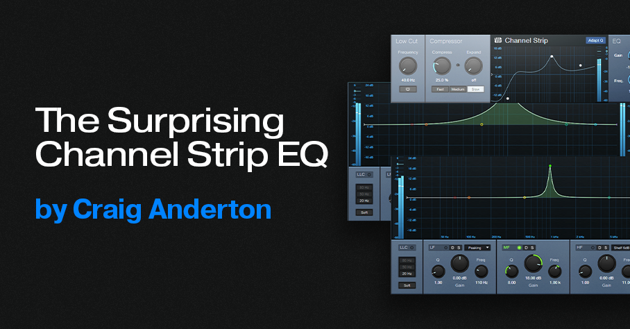
The Surprising Channel Strip EQ
Announcement: Version 1.4.1 of The Huge Book of Studio One Tips and Tricks is a free update to owners of previous versions. Simply download the book again from your PreSonus account, and it will be the most recent version. This is a “hotfix” update for improved compatibility with Adobe Acrobat’s navigation functions. The content is the same as version 1.4.
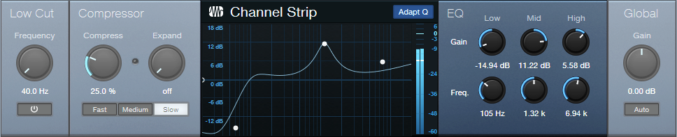
Studio One has a solid repertoire of EQs: the Fat Channel EQs, Pro EQ3, Ampire’s Graphic Equalizer, and the Autofilter. Even the Multiband Dynamics can serve as a hip graphic EQ. With this wealth of EQs, it’s potentially easy to overlook the Channel Strip’s EQ section (fig. 1). Yet it’s significantly different from the other EQs.
Back to the 60s
In the late 60s, Saul Walker (API’s founder) introduced the concept of “proportional Q” in API equalizers. To this day, engineers praise API equalizers for their “musical” sound, and much of this relates to proportional Q.
The theory is simple. At lower gains, the bandwidth is wider. At higher gains, it becomes narrower. This is consistent with how we often use EQ. Lower gain settings are common for tone-shaping. Increasing the gain likely means you want a more focused effect.
The concept works similarly for cutting. If you’re applying a deep cut, you probably want to solve a problem. A broad cut is more about shaping tone. Also, because cutting mirrors the response of boosting, proportional Q equalizers make it easy to “undo” equalization settings. For example, if you boosted drums around 2 kHz by 6 dB, cutting by 3 dB produces the same curve as if the drums had originally been boosted by 3 dB.
Proportional Q also works well with vocals and automation. For less intense parts, add a little gain in the 2-4 kHz range. When the vocal needs to cut through, raise the gain to increase the resonance and articulation.
The Channel Strip’s Adapt Q button converts the response to proportional Q. Let’s look at how proportional Q affects the various responses.
High and Low Stages
The High band is a 12 dB/octave high shelf. In fig. 2, the Boost is +15 dB, at a frequency of 2.5 kHz. The top image shows the EQ without Adapt Q. The lower image engages Adapt Q, which increases the shelf’s resonance.
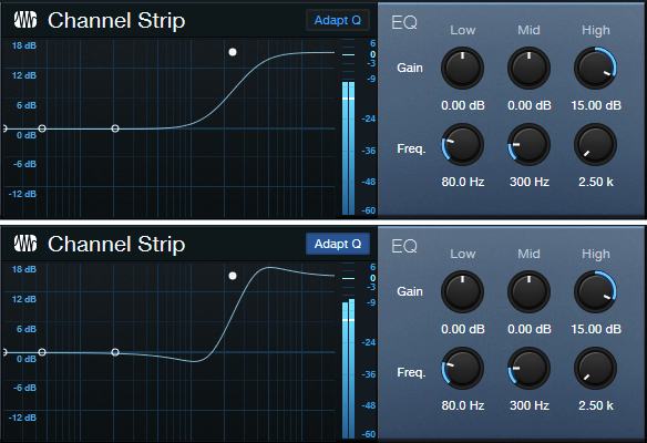
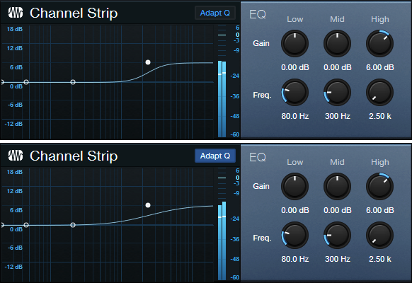
Fig. 3 shows what happens with 6 dB of gain. With Adapt Q enabled, the Q is actually less than the corresponding amount of Q without Adapt Q.
Cutting flips the curve vertically, but the shape is the same. With the Low shelf filter, the response is the mirror image of the High shelf.
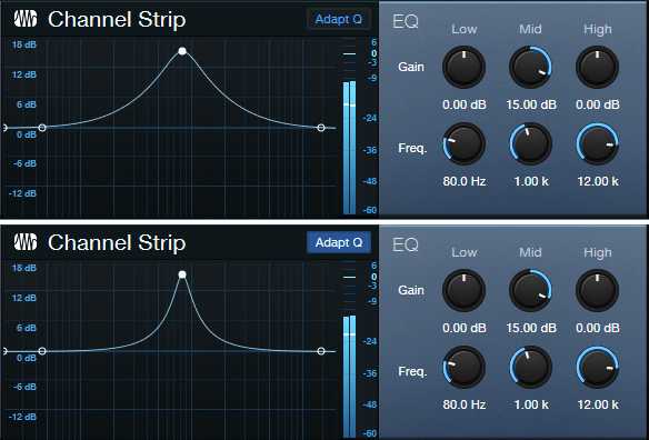
Midrange Stage
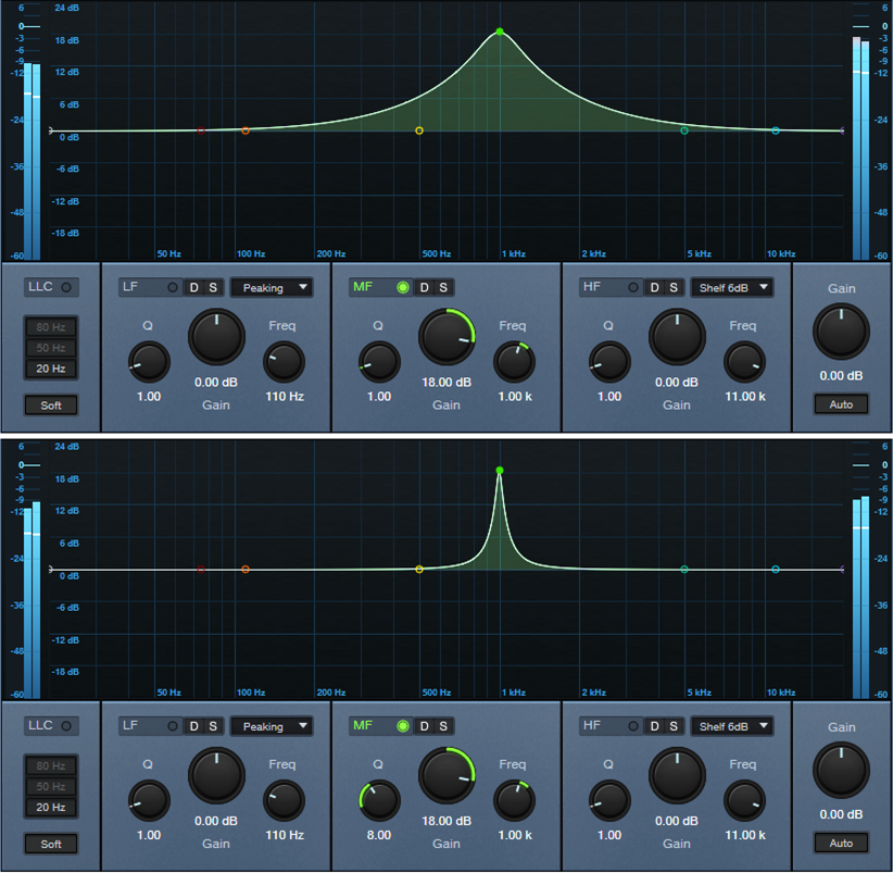
The Midrange EQ stage has variable Gain and Frequency. There’s no Q control, but the filter works with Adapt Q to increase Q with more gain or cut (fig. 4).
With 6 dB Gain, the Q is essentially the same, regardless of the Adapt Q setting (fig. 5).

Finally, another Adapt Q characteristic is that the midrange section’s slope down from either side of the peak (called the “skirt”) hits the minimum amount of gain at the same upper and lower frequencies, regardless of the gain. This is different from a traditional EQ like the Pro EQ3, where the skirt narrows with more Q (fig. 6).
Perhaps best of all, the Channel Strip draws very little CPU power. So, if you need more stages of EQ, go ahead and insert several Channel Strips in series, or in parallel using a Splitter or buses. And don’t forget—the Channel Strip also has dynamics 😊!
Set Up the Quantum Interface Preamps with One Track
A single Automation track can set up a session’s preamp levels and phantom power in the Quantum interface, as well as the older Studio 192. So, you can stop taking the time to reset preamp levels if you do lots of different sessions—let Studio One set up the preamps whenever you call up a specific song.
For example, I mostly use three vocal mics. However, their optimum gain settings vary for narration, music vocals, or recording my main background vocalist—who needs different gain settings depending on whether she’s doing upfront vocals, or ooohs/ahhhs.
To call up specific preamp levels for different songs, simply create an automation track (or tracks) at the song’s beginning. Then, when you first hit record, the track sets up levels and (with Quantum and Studio 192) phantom power on/off for up to 8 channels. The next time you call up that song, the mics will be at the right levels, with phantom power set as desired. Here’s how to do it.
1. In Universal Control, under MIDI Control, select Internal. Or, choose Enabled if you also want to be able to control Quantum from an external controller.
2. Choose Studio One > Options (Windows) or Preferences (macOS), and select External Devices.
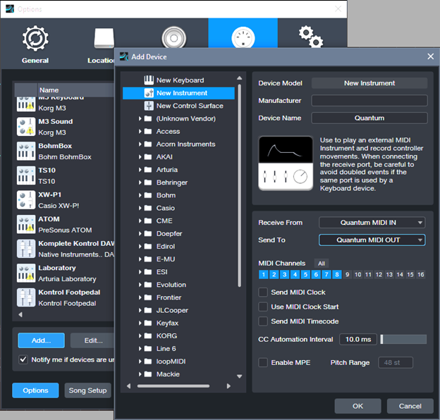
3. Select Add. Choose New Instrument.
4. For Receive From, choose Quantum MIDI In. For Send To, choose Quantum MIDI Out. Also tick MIDI Channels 1 – 8 (fig. 1). Then, click OK.
5. Create an Automation track. To show automation, type keyboard shortcut A.
6. From the track’s automation drop-down menu, click on Add/Remove. In the right pane, unfold the External Devices folder, then unfold the folder for the Channel that corresponds to the preamp you want to control (Channel 1 = Preamp 1, Channel 2 = Preamp 2…Channel 8 = Preamp 8). See fig. 2.
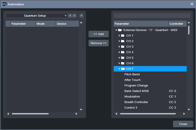
7. For each preamp you want to set up, add CC7 (this controls preamp volume) and CC14 (controls phantom power). For example, I typically set up channels 6, 7, and 8. After adding these continuous controllers, the Automation menu’s right side looks like fig. 3 (except with your specific channel numbers). Click on Close after making your selections.

8. To set up the preamp levels, choose the parameter you want to program in the Automation track’s drop-down menu. Note that in the documentation, the phantom power control settings are reversed. The correct values for CC14 are 0 to 63 = Off, and 64 to 127 = On. To set the preamp level, with Universal Control open, adjust the envelope for the desired preamp gain reading (you can also see the level on the Quantum’s display).
9. Set the initial level and phantom power parameter values for the chosen preamps. Now your automation track will reproduce those settings, exactly as programmed, the next time you open the song. Given that I do voiceover or narration for at least one video a week, I can’t tell you how much time that saves—I load my narration template, and don’t even have to think about adjusting levels before hitting record.
Getting Fancy
A cool trick is to reserve a song’s first measure for doing the setup. Turn on phantom power at the song start, but fade up the volume to the desired level after the phantom power is on. That avoids power-on spikes from the mics. However, when adjusting the level envelope, the preamp knobs change only if you adjust the left-most node. So, set the preamp level you want with this node, then move it to the right on the timeline. Create another node at 0 that fades up to the node you moved, which sets the final volume.
Another trick is to have more than one automation track. For example, on most songs I have a setup track for me, and a setup track for the background singer. When she does overdubs, I turn my automation track to Off, and set her automation track to Read so it sets her levels.
Coda: Windows Meets Thunderbolt
The first time I tried Quantum on a Mac, it worked perfectly. With Windows, well…it’s Windows. My computer is a PC Audio Labs Rok Box (great machine, by the way) with dual Thunderbolt 3 ports. I used Apple’s TB3-to-TB2 adapter—no go. I found a new Thunderbolt driver for the motherboard, and asked PC Audio Labs tech support about whether I should install it. They advised doing so, and said if I had problems, they’d bail me out. But after installation, the Quantum’s power button’s color was still Unhappy Red instead of Happy Blue. I was about to contact support again, but stumbled on a program in the computer called Thunderbolt Control Center. I opened it, which showed Quantum was connected—but I hadn’t given the computer “permission” to connect. So, I gave permission. With its new-found freedom, the Quantum burst into its low-latency glory.
The moral of the story: Thunderbolt has many variables on Windows than macOS. But as with life itself, perseverance furthers.
The “Drenched” Chorus
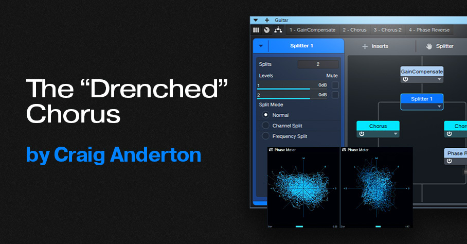
Studio One’s chorus gives the “wet” sound associated with chorus effects. But I wanted a chorus that went beyond wet to drenched—something that could swirl in the background of a thick arrangement, and shower the stereo field like a sprinkler system. Check out the audio example: the first part is the Drenched Chorus, and the second part is the standard Chorus.
This FX Chain for Studio One Professional (see the download link at the end) supercharges the wet sound by inserting two choruses in parallel, and reversing the phase for one of them (fig. 1). This cancels any dry sound, leaving only the animation from the stereo chorus. A Mixtool provides the phase reversal. Another Mixtool at the input adds gain, to compensate for the level that’s lost through phase cancellation.
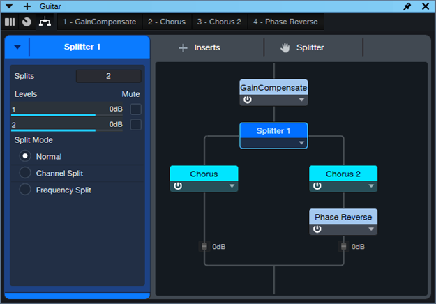
The Choruses are essentially set to the default preset, but with Low Freq at minimum and High Freq at maximum for the widest frequency response. Fig. 2 uses a phase meter to compare the Drenched Chorus (left) with the standard Chorus (right), playing the same section of a guitar part. Note how the Drenched Chorus puts a lot of energy into the sides, which accounts for the big stereo image. Meanwhile, the center has less level than the standard chorus, due to any vestiges of dry signal being removed.
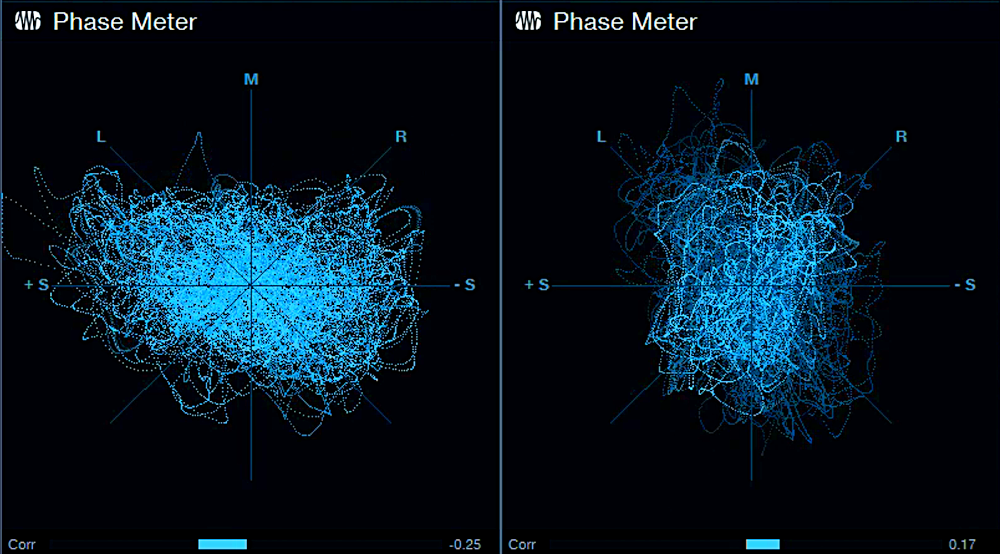
This effect is designed for stereo playback, but note that in fig. 2, the Drenched Chorus’s correlation is negative. Normally you want to avoid this, because audio with negative correlation will cancel when played back in mono. However, the correlation swings wildly between positive and negative, so it’s not much of an issue. With mono playback, all that happens is a slight level loss due to occasional negative correlations. The effect still sounds like a chorus, although of course you lose the cool stereo effects.
How to Use It
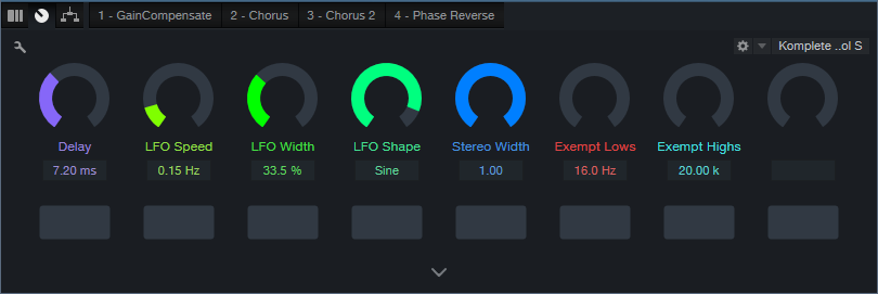
Download the FX Chain, and drag it into a channel’s insert. The Macro Controls (fig. 3) affect only Chorus 2. Here’s what they do:
- Delay: Set this to 9.00 for maximum cancellation. The sound is somewhat like a combination of chorusing and flanging. Offsetting from this time increases the chorus effect. The maximum Drenched Chorus effect occurs between approximately 7 and 11 ms.
- LFO Speed: I prefer settings below 0.30 Hz, but higher settings have a bit of a rotating speaker vibe.
- LFO Width: More Width increases the chorusing effect. If you turn this up, I recommend keeping LFO Speed below 0.30 Hz.
- LFO Shape: Setting this to Triangle uses the same shape as the other Chorus. Sine gives a subtly different sound.
- Stereo Width: Extends the stereo image outward when turned clockwise.
- Exempt Lows: This turns up the Low Freq filter, which reduces cancellation at those frequencies. Use this when you want more of the direct sound instead of maximum drenching.
- Exempt Highs: This turns down the High Freq filter, which reduces cancellation at those frequencies. Personally, I leave both controls all the way down for maximum moisture, but turn them up if you want the track to swim a little less in the background.
Download the FX Chain below!